Diffusion and Osmosis, Explained
After reading this you will be able to predict which way particles flow across a wall, estimate how high a solution climbs under osmotic pressure, and explain why all of it happens without any force pushing the particles.
What the model shows
Split a tank down the middle with a wall. Put water molecules and salt particles on each side, then let everything jostle at random. Nothing pulls the particles anywhere. Each one takes a random step every tick. Yet the concentrations equalise every time. That is the whole idea, and it is worth pausing on: the drift toward balance is a counting fact, not a force.
The tool runs two cases side by side. With a fully permeable wall, both species cross freely and mix until each side holds about the same number of each. That is plain diffusion. With a semipermeable wall, the small solvent particles slip through the pores but the large solute particles cannot. Now something more specific happens. Water drifts toward the saltier side and raises its level. That net water flow is osmosis.
Here is the hook. Suppose the left half starts with 200 water and 40 salt, and the right half starts with 200 water and 0 salt. The salt cannot move, so it stays 40 on the left forever. But the water redistributes. When the system settles, the two sides carry water in proportion to their total capacity for it, and the left side ends up holding more water than it began with. The level on the salty side rises. No pump, no attraction. Just more ways to arrange things.
When this picture applies and when it does not
Use this model to build intuition for three claims: diffusion moves particles from high to low concentration on average, a semipermeable wall converts a solute imbalance into a water flow, and the flow stops when a height difference produces enough back pressure to cancel it.
Do not read exact chemistry off the screen. The particles here are hard markers taking uncorrelated random steps. Real water molecules interact, form hydrogen bonds, and carry charge if the solute is an ion. The tool also ignores temperature gradients and treats the membrane as a perfect sieve with a sharp size cutoff. Real membranes leak, and real solutes drag water with them. Treat the numbers as a clean statistical cartoon that gets the direction and the qualitative size right.
The same random-walk logic drives many models on this site. If you want to see the underlying molecular motion that produces diffusion, watch speeds settle in Ideal Gas and Maxwell-Boltzmann, then see what happens when diffusing chemicals also react in Reaction-Diffusion Patterns.
The math behind the drift
Start with why diffusion has a direction at all. Suppose N water particles wander between a left cell and a right cell, and each is equally likely to be on either side. The number on the left follows a binomial distribution. The most probable split is 50-50 because that arrangement has the most microstates. With N = 400, the number of ways to put 200 on the left is about 10^{119} times larger than the number of ways to put all 400 on one side. That ratio is the entire reason mixing looks one-way.
Diffusion at the level of concentration c(x, t) obeys Fick's law and the diffusion equation:
Here c is concentration, t is time, x is position, and D is the diffusion coefficient (area per unit time). Wherever concentration is curved (a peak), the second derivative is negative and the peak falls. Wherever it dips, the dip fills. Flat concentration is the only steady state, which is exactly equalisation.
For osmosis, the water climbs until its weight pressure balances the tendency to keep diluting. For a dilute solution, van 't Hoff's law gives the balancing pressure:
Here \Pi is the osmotic pressure, c is the molar concentration of solute particles that cannot cross, R = 8.314\ \text{J mol}^{-1}\text{K}^{-1} is the gas constant, and T is absolute temperature in kelvin. Notice the form: it is identical to the ideal gas law P = (n/V) R T. The trapped solute behaves like a gas pressing outward, and water flows in to relieve that pressure.
A worked example with the demo numbers
Water redistribution with a semipermeable wall
Take the default setup: 200 water and 40 salt on the left, 200 water and 0 salt on the right, with a semipermeable wall. Salt is trapped, so left keeps 40 and right keeps 0.
- Total water to distribute:
200 + 200 = 400. - Total particles left:
200 + 40 = 240. Total right:200 + 0 = 200. Grand total:440. - At equilibrium the free water arranges so that the water concentration is equal on both sides. Water settles in proportion to each side's share of the total particle count: left share 240/440 = 0.5455, right share 200/440 = 0.4545.
- Water on the left: 400 \times 0.5455 = 218.2. Water on the right: 400 \times 0.4545 = 181.8.
- The left side gained about
18water particles it did not start with. That extra volume is the level rise. The right side dropped by the same 18.
Check the concentrations. Left solute fraction: 40 / (218.2 + 40) = 0.1550. Right solute fraction: 0 / 181.8 = 0. The salt is still only on the left, but the water is now evenly concentrated because both sides carry water at the same density relative to space. The system reached balance by moving water, not salt.
An interactive to feel the balance point
Reading the results on screen
Three readouts matter. First, the particle counts per side. Watch the crossing species approach equal concentration and the trapped species stay put. Second, the level difference, which is the height the water climbs on the salty side. Third, the shape of the approach curve: steep early, flat late.
The level difference is your osmotic pressure gauge. It stops rising when the extra weight of the raised column exactly opposes the diffusive tendency of water to keep entering. If you double the trapped salt, van 't Hoff says the balancing pressure doubles, so the equilibrium level difference roughly doubles too, at least while the solution stays dilute.
| Trapped salt | Left water | Right water | Level difference |
|---|---|---|---|
| 0 | 200 | 200 | 0 |
| 20 | 209.5 | 190.5 | 19.0 |
| 40 | 218.2 | 181.8 | 36.4 |
| 100 | 240.0 | 160.0 | 80.0 |
| 200 | 266.7 | 133.3 | 133.3 |
Common mistakes
Do not say the salt is "pulling" the water in. Nothing attracts anything here. Water enters the salty side because a smaller fraction of its molecules there are free to leave, so the outbound rate is lower than the inbound rate until the level difference evens the two rates. The imbalance is in the counting, not in a force.
A second error is expecting the trapped solute to spread. It cannot cross the wall, so its per-side count never changes with a semipermeable membrane. Only its concentration changes, and only because water moves.
A third error is reading the flat part of the curve as "no motion." At equilibrium particles still cross both ways at a furious rate. The net flow is zero because the two directions balance. Turn off the wall entirely and you get pure diffusion, where the two species mix and no permanent level difference forms.
Finally, do not extend van 't Hoff's law to strong solutions. At high concentration the linear form \Pi = c R T overpredicts, because particle interactions and crowding matter. The tool's dilute-limit numbers only track the law while c stays small.
Related simulations
The random-walk core here shows up all over statistical physics. To watch particles aggregate one wandering step at a time, try the Crystal Growth Simulator. To see a fluid change phase as it cools, run Molecular Dynamics: Phases of Matter. For a lattice version of the same order-from-randomness idea, the Ising Model Ferromagnet shows domains forming and melting, and Percolation finds the tipping point where a random path first spans a grid. If you enjoy chemistry that refuses to settle, the Belousov-Zhabotinsky Reaction oscillates instead of equalising, and the Flame Simulator paints living fire.
Frequently asked questions
Why does diffusion have a direction if every step is random?
Because there are vastly more ways to be spread out than clustered. With 400 particles the even 200-200 split outnumbers the all-on-one-side arrangement by about a factor of 10^{119}. Random steps land you in the arrangement with the most ways to occur, and that is the mixed state.
What is the difference between diffusion and osmosis?
Diffusion is any species spreading to even out its own concentration. Osmosis is a special case: the solvent diffusing through a membrane the solute cannot cross, which produces a net flow of solvent toward the saltier side and a rise in its level.
How high does the water actually climb?
Until the pressure of the raised column equals the osmotic pressure \Pi = c R T. In the model the level difference tracks the trapped solute count: 40 salt gives a difference of about 36 water units, 100 salt gives 80, 200 salt gives 133, as the table shows.
Does osmosis stop, or does water keep flowing forever?
Net flow stops at equilibrium. Individual particles keep crossing both ways at equal rates, so the level holds steady while the traffic continues.
Is this how plant cells stay firm?
Yes, in outline. A plant cell holds dissolved solutes the wall traps, so water enters and presses the membrane against the cell wall. That turgor pressure is the same osmotic pressure this model measures as a height.
Related tools
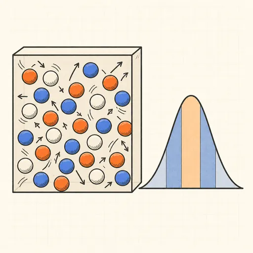
Ideal Gas & Maxwell–Boltzmann
Bounce hard-disc molecules in a box and watch their speeds settle into the Maxwell–Boltzmann distribution.
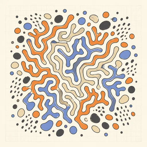
Reaction–Diffusion Patterns
Grow coral, spots and zebra stripes from two virtual chemicals with the Gray–Scott model.
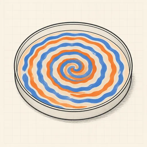
Belousov–Zhabotinsky Reaction
Watch an oscillating chemical medium organize itself into rotating spiral waves.

Crystal Growth Simulator
Grow branching fractal crystals one wandering particle at a time with diffusion-limited aggregation.
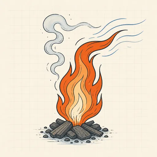
Flame Simulator
Paint fire and shape a living flame with fuel, cooling, wind and turbulence.
Ising Model Ferromagnet
Flip a grid of spins at any temperature and watch magnetic domains freeze in or melt at the critical point.