The Ising Model, Explained
After reading this you will know how a grid of magnetic spins decides to line up or scramble, why there is a sharp temperature where order suddenly appears, and how to read magnetisation and energy as they cross that point.
What the model is
The Ising model is the simplest picture of a magnet that still behaves like a real one. Take a square grid. Put a tiny arrow on each site that can only point up (+1) or down (-1). That arrow is a spin. Each spin prefers to match its four nearest neighbours, because matching lowers the energy. Nothing else happens: no motion, no chemistry, just a field of arrows nudging each other.
Run it cold and the arrows agree. Whole regions turn the same way, and the grid becomes magnetised. Run it hot and thermal kicks flip spins at random, so the up and down counts even out and the net magnetisation drops to zero. The interesting part sits between those extremes. On a 2D square lattice the change from ordered to disordered happens at a single temperature near 2.269, and it happens sharply. That abrupt change is a phase transition, the same kind of event as water freezing.
Here is the hook. Cool a real ferromagnet below its Curie temperature and it can hold a permanent magnetic moment. Heat it past that point and the moment vanishes. Iron does this at about 1043 kelvin. The Ising model reproduces that behaviour from one rule (spins like their neighbours) and one competing effect (temperature scrambles them), which is why it appears in almost every statistical physics course.
When to use it, and when not
Use the Ising model when you want to understand collective behaviour: how local rules that each site follows add up to a global property that no single site carries. Magnetisation is the classic example, but the same math describes lattice gases, binary alloys where two metals prefer to segregate, and simplified neural and opinion models. If your question is "when does local agreement turn into global order," this is the right toy.
Do not read it as a literal picture of iron. The spins here sit frozen on a grid and interact only with four neighbours. Real magnetic materials have moving atoms, three dimensions, long-range dipole forces, and quantum spins that can point in any direction. The 2D Ising model also gets some numbers wrong on purpose: its critical exponents differ from those in three dimensions, and the exact critical temperature 2.269 is specific to the 2D square lattice with equal couplings.
The 2D Ising model is one of the few interacting many-body systems solved exactly. Lars Onsager published the solution in 1944. That exact answer is why the simulation is worth trusting: you can check the temperature it produces against a known number instead of guessing.
The energy rule and the flip probability
Two formulas run the whole simulation. The first is the energy of a configuration of spins.
Here s_i = \pm 1 is the spin at site i. The notation \langle i,j \rangle means you sum over each neighbouring pair once. J \gt 0 is the coupling strength; a positive J makes aligned neighbours lower the energy, which is the ferromagnetic case. H is an external field that tries to pull every spin one way. If two neighbours agree, their term contributes -J; if they disagree it contributes +J. Order is cheap, disorder is expensive.
The second formula decides whether a proposed flip actually happens. This is the Metropolis rule. Pick a spin, compute how much the energy would change if you flipped it, call that \Delta E, then accept with this probability.
T is temperature and k_B is Boltzmann's constant, which the simulation sets to 1 so temperature is measured in units of J/k_B. Read the rule plainly: any flip that lowers energy (\Delta E \le 0) is always accepted, and a flip that raises energy is accepted only sometimes, with a chance that shrinks as the energy cost grows or the temperature drops. That single exponential is what lets the grid climb out of bad arrangements at high temperature and freeze into good ones at low temperature.
A worked example you can reproduce
Flipping one spin on a 2D grid
Load the tool with its default settings and pause on a single spin. Suppose the spin points up (s = +1) and all four of its neighbours point up too. With J = 1 and no field (H = 0), flipping this spin from +1 to -1 costs energy because it now disagrees with all four neighbours.
- Energy change for flipping one spin: \Delta E = 2 J s \sum_{\text{neighbours}} s_j. The sum of neighbours is +4, and s = +1, so \Delta E = 2 \cdot 1 \cdot 1 \cdot 4 = 8.
- At a cold temperature T = 1.0, the acceptance probability is e^{-8/1} = e^{-8} \approx 0.000335. That flip almost never happens, so the aligned block stays put.
- At a hot temperature T = 5.0, the same flip has probability e^{-8/5} = e^{-1.6} \approx 0.2019. Now roughly one in five such flips is accepted, so aligned blocks keep tearing apart.
- Right near the critical point T = 2.269, the probability is e^{-8/2.269} = e^{-3.526} \approx 0.02951. Rare, but not negligible, which is exactly why domains of every size coexist there.
The factor of 2 appears because flipping the spin does not just remove the old alignment energy, it adds the opposite. Each satisfied bond worth -J becomes a broken bond worth +J, a swing of 2J per neighbour.
Reading magnetisation and energy
The tool reports two running numbers. Magnetisation per spin is the average of all spins, m = \frac{1}{N}\sum_i s_i, so it runs from -1 (all down) to +1 (all up). Energy per spin is E/N from the first formula. Watch how both change as you drag temperature.
Cold, the magnetisation sits near |m| \approx 1 and the energy sits near its minimum of -2J per spin (each spin shares two bonds, each worth -J). Hot, magnetisation hovers near 0 and energy climbs toward 0 because half the bonds are broken on average. The curve of |m| against temperature stays high, then plunges to zero over a narrow window around 2.269. The exact solution gives the shape below.
The energy curve tells the same story from the other side. Its steepest slope marks the point where the most bonds are breaking per degree of heating, and that slope is the specific heat. In an infinite system the specific heat diverges at 2.269. On a finite grid it shows up as a sharp but finite peak, taller when the grid is bigger.
Track |m| rather than m when scanning temperature. Below the critical point the whole grid can flip between all-up and all-down over a long run, so the signed average can average out to near zero even though the material is fully ordered at every instant.
What happens at the critical point
At exactly 2.269 the domains stop having a single typical size. You see patches within patches within patches, and the pattern looks statistically the same whether you zoom in or out. This is scale invariance, and it is the reason critical phenomena are studied so hard: near a critical point the microscopic details stop mattering and whole classes of systems share the same exponents.
Concretely, the correlation length (the distance over which two spins tend to agree) grows without bound as T approaches 2.269. Below the critical temperature it is finite because domains have a size. Above it, it is finite because agreement decays fast. Only at the transition does it diverge, which is why a small grid never shows a perfectly sharp jump: your grid is smaller than the correlation length wants to be.
Common mistakes
The errors below all come from expecting the wrong number or the wrong shape.
- Reading before equilibrium
- The Metropolis walk needs time to settle, and it needs the most time right near
2.269, where flips propagate slowly. If you snap a reading one sweep after changing temperature, the magnetisation you record is a leftover from the old temperature, not the new one. - Confusing the field with temperature
- An external field H also aligns spins, but it does it by tilting the energy, not by adding order for free. A strong field can force |m| \approx 1 even when hot, which hides the phase transition entirely. Set H = 0 to see the spontaneous transition.
- Expecting a perfectly vertical jump
- The exact curve is vertical only for an infinite lattice. On a 64 by 64 grid the drop is smeared over a window of roughly \pm 0.1 in temperature, and the apparent critical temperature you measure sits slightly above
2.269. That shift shrinks as the grid grows. - Comparing to a real Curie temperature in kelvin
- The
2.269here is in units of J/k_B. To turn it into kelvin you need the real coupling J of a specific material, and even then the 2D value differs from the 3D one. The number is a ratio, not a laboratory reading.
Related tools on this site
The Ising model is one of several small worlds where local rules build global structure. To see thermal probability from the other direction, watch molecules sort themselves in the Ideal Gas & Maxwell-Boltzmann simulation, where the same Boltzmann factor e^{-E/k_B T} sets the speed distribution. For a sharp threshold driven purely by geometry rather than temperature, try Percolation, whose spanning transition is a close cousin of the Ising critical point. To watch matter reorganise as it cools, the Molecular Dynamics: Phases of Matter tool takes a Lennard-Jones fluid from gas to crystal. And for pattern formation from a different rule set, see the Reaction-Diffusion Patterns tool.
Frequently asked questions
Why is the critical temperature 2.269 and not something round?
Onsager's exact solution gives T_c = 2 / \ln(1 + \sqrt{2}) in units of J/k_B. Evaluate it: \sqrt{2} \approx 1.4142, so \ln(2.4142) \approx 0.8814, and 2 / 0.8814 \approx 2.269. The odd number is a consequence of the square lattice geometry.
Does the model ever settle down completely?
No, and it should not. Even deep in the cold phase, thermal fluctuations flip occasional spins and heal them. What settles is the average: |m| and energy per spin fluctuate around fixed values once the grid reaches equilibrium. The fluctuations are largest near 2.269.
What does a positive versus negative coupling mean?
A positive J makes neighbours want to agree, the ferromagnetic case shown here. A negative J makes them want to disagree, the antiferromagnetic case, which on a square lattice produces a checkerboard ground state instead of uniform domains.
Why does the flip cost use a factor of 2?
Flipping a spin turns each satisfied bond (energy -J) into a broken one (energy +J), a change of 2J per neighbour. With four aligned neighbours the total swing is 8J, which is the \Delta E = 8 used in the worked example.
How big should the grid be?
Bigger grids show a sharper transition and a taller specific-heat peak, but they run slower because each sweep touches every site. A grid of 64 by 64 (4096 spins) already shows clear domains and a visible transition while updating fast enough to watch live.
Related tools
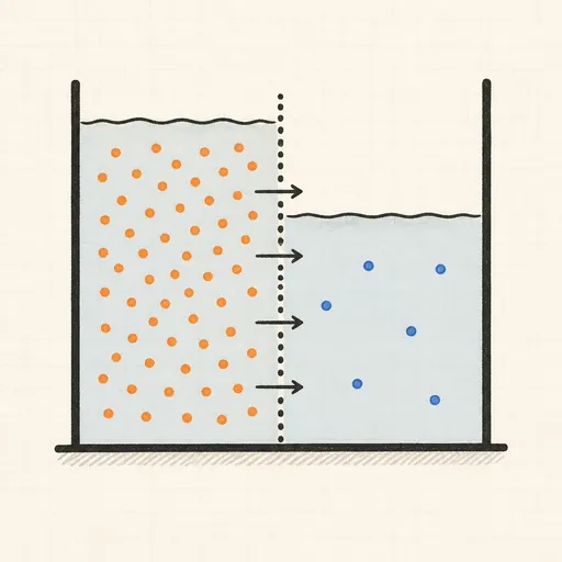
Diffusion & Osmosis
Split a tank with a semipermeable wall and watch particles diffuse and water flow to equalise concentration.
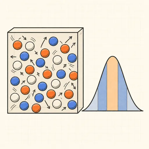
Ideal Gas & Maxwell–Boltzmann
Bounce hard-disc molecules in a box and watch their speeds settle into the Maxwell–Boltzmann distribution.
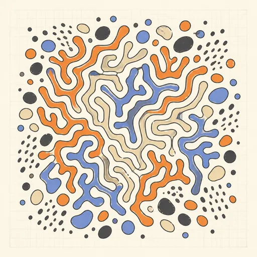
Reaction–Diffusion Patterns
Grow coral, spots and zebra stripes from two virtual chemicals with the Gray–Scott model.
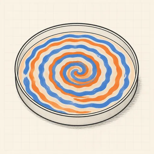
Belousov–Zhabotinsky Reaction
Watch an oscillating chemical medium organize itself into rotating spiral waves.
Crystal Growth Simulator
Grow branching fractal crystals one wandering particle at a time with diffusion-limited aggregation.

Flame Simulator
Paint fire and shape a living flame with fuel, cooling, wind and turbulence.