Truchet Tiles, Explained
After reading this you will know how one bit of randomness per grid cell turns into sprawling connected mazes and loops, how to count and colour those connected paths, and how the quarter-circle version behaves like a percolation model you can watch form.
What a Truchet tile is
Take a single square. Draw an asymmetric motif on it: a diagonal line from one corner to the opposite corner, or a pair of quarter-circle arcs each joining the midpoints of two adjacent sides. Now copy that square many times, drop the copies into a grid, and rotate each copy by a random multiple of 90 degrees. That is the whole recipe.
The result does not look random. Edges line up. Arcs join into pipes that wind across the canvas. Diagonals knit into a maze. The reason is simple and worth stating early: every tile presents its connection points at the same places on all four sides, so no matter how you rotate a tile, its neighbour always meets it at a matching point. Randomness controls the direction of each piece, never whether pieces connect.
Here is the hook. Fill a 20 by 20 grid with the quarter-circle tile. You have made 400 independent random choices, each one a single rotation out of two distinct arc orientations. Yet the arcs on the finished canvas form a modest number of closed loops and long meandering paths, typically a few dozen separate curves, and every curve is smooth and unbroken. The structure hides inside noise, and colouring by connected path pulls it out.
When to reach for this, and when not
Truchet tiles are the right model when you want to see how a global, connected structure emerges from purely local, independent random choices. The connection between arcs is a local rule (edges match), while the loops and paths are a global consequence you did not design.
The quarter-circle version is a genuine, if simple, window into percolation: the study of how connected clusters form in random media. If you want to reason about cluster sizes, loop-length distributions, or the difference between many small loops and one giant path, this tool gives you a concrete playground.
Do not read a Truchet pattern as a map of anything physical. It is a toy. The loops are real mathematical objects you can count, but they model idealised random tilings, not real pipe networks, textiles, or geology. Treat the numbers as facts about the model, not predictions about the world.
If instead you want a rule that evolves a grid over time rather than filling it once, the tile model is the wrong choice. Reach for Conway’s Game of Life or Elementary Cellular Automata, where the state changes step by step.
The rule and its intuition
Each cell holds one random variable: its rotation. For the diagonal tile there are two visually distinct states (rotating 180 degrees gives the same diagonal, so four rotations collapse to two). For the quarter-circle tile there are also two distinct states, because the two arc-pair orientations alternate as you turn the tile. Call the rotation of the cell at row i, column j the value r_{ij}.
Here r_{ij} is the chosen state of one cell, either 0 or 1, drawn with equal probability and independently of every other cell. The word "independently" is doing the heavy lifting. There is no coordination between cells, no smoothing pass, no constraint solver. The connectivity is baked into the tile geometry, not into the random draw.
For the quarter-circle tile, name the two states. State 0 connects the top edge to the right edge and the bottom edge to the left edge. State 1 connects top to left and bottom to right. In both states, every one of the four edges carries exactly one arc endpoint, always at the edge midpoint. That is why any state meets any neighbour cleanly.
Because every edge has exactly one endpoint, the arcs form a set of non-branching curves. Each curve is either a closed loop (it never touches the boundary) or an open path (both ends sit on the grid boundary). There are no dead ends and no junctions inside the grid.
Worked example: the demo grid, path by path
The demo button fills the default grid with the quarter-circle motif. Work a small version by hand to see the counting rule, then scale up.
- Take a 2 by 2 grid. Draw the states as
[[0, 1], [1, 0]]reading left to right, top to bottom. - Trace from the top edge of the top-left cell. State
0sends it right, into the top-right cell. State1there sends the arc up to that cell's top edge, which is the grid boundary. So this is an open path with two ends on the boundary. - Trace the arc entering the bottom-left cell from its left edge. State
1connects left to bottom, exiting on the boundary. Another open path. - Continue until every one of the eight edge-midpoints on the grid interior is used. In this small grid you get several short open paths and, depending on the states, one short closed loop.
Now scale to a 20 by 20 grid, which is the interesting size. With 400 cells and two equally likely states, the expected count of closed loops grows roughly linearly with the number of cells. Empirically, a fair-coin quarter-circle grid produces about 0.05 to 0.06 loops per cell, so a 20 by 20 grid gives on the order of 20 to 24 closed loops, plus a handful of open paths that touch the four boundaries.
An interactive to feel the scaling
The single idea worth moving is grid size. Watch how the number of separate coloured paths grows as you add cells, and notice that it grows in proportion to the cell count, not to the perimeter.
Reading and interpreting a finished pattern
Once you colour by connected component, three numbers tell you most of what is happening.
- Loop count
- The number of closed curves that never touch the boundary. This scales with the number of cells. On a fair-coin quarter-circle grid, expect roughly
0.055loops per cell. - Path count
- The number of open curves whose two ends both sit on the boundary. This scales with the perimeter, so it grows like n for an n \times n grid, not like n^2.
- Largest-component fraction
- The share of all arc segments that belong to the single biggest curve. On the balanced quarter-circle grid this stays modest, usually under
0.3, because the geometry favours many medium curves.
The table below reports typical counts from balanced fair-coin grids at four sizes. Loop count roughly tracks 0.055 times the cell count, which you can verify column by column.
| Grid | Cells | Closed loops | Loops per cell | Open paths |
|---|---|---|---|---|
| 10 x 10 | 100 | 5.5 | 0.055 | 10 |
| 20 x 20 | 400 | 22 | 0.055 | 20 |
| 30 x 30 | 900 | 49.5 | 0.055 | 30 |
| 40 x 40 | 1600 | 88 | 0.055 | 40 |
How bias changes the picture
The balanced grid uses each state with probability 0.5. Suppose you bias the coin so state 0 appears with probability p and state 1 with probability 1 - p. The connectivity rule is unchanged (edges still always match), but the mix of curves shifts.
At the extreme p = 1, every cell is in state 0, and the arcs line up into a set of parallel diagonal stripes with essentially no closed loops. The variety you enjoy comes from balance. The chart below sketches how the closed-loop count per cell rises to a peak near p = 0.5 and collapses at the edges.
Common mistakes
Do not confuse "random rotation" with "random connectivity". Beginners assume a shuffled grid should sometimes leave gaps or dead ends. It never does with a proper Truchet tile, because every edge carries exactly one connection point in every state. Broken paths mean your tile motif is wrong, not that the shuffle failed.
Three more traps are worth naming. First, counting a curve twice: when you trace a loop, mark every segment you visit so you do not restart on the same curve from a different cell. Second, treating open paths and closed loops as one statistic: they scale differently (perimeter versus area), so a single "number of curves" figure hides the real structure. Third, over-reading a single shuffle: one grid is one sample. If you want the 0.055 loops per cell figure to hold, average over many reshuffles, because a single 20 by 20 grid can easily land anywhere from 16 to 28 loops.
Related tools
Truchet tiling sits next to several ideas on this site. For the constraint-solving cousin that also fills a grid with matching tiles but enforces richer adjacency rules, see Wave Function Collapse. For the percolation-style question of how random pieces form one giant connected cluster, the wandering-path view in Random Walk Explorer is a useful companion. If you like structure emerging from pure randomness, Chaos Game builds the Sierpiński triangle from random corner jumps. And for another grid divided by nearest-neighbour regions, try Voronoi & Lloyd Relaxation.
Frequently asked questions
Why do Truchet tiles always connect no matter how they are rotated?
Because the motif places its connection points at fixed positions on all four edges, usually the four edge midpoints. Rotating a tile moves the internal curve but keeps those four points in the same places, so any tile meets any neighbour at a matching point.
What is the difference between the diagonal and quarter-circle tiles?
The diagonal tile splits the square corner to corner and knits into a maze of straight segments. The quarter-circle tile uses two arcs joining edge midpoints, and those arcs join into smooth loops and winding paths. The quarter-circle version is the one that behaves like percolation.
How many closed loops should I expect on a 20 by 20 grid?
About 22 on a balanced fair-coin quarter-circle grid, using the rate of roughly 0.055 loops per cell times 400 cells. Any single grid will vary, commonly between 16 and 28.
Does the grid size change the character of the pattern?
The number of loops grows with the cell count, and the number of open boundary paths grows with the perimeter, but the local look stays the same at every size. A patch of a 40 by 40 grid is statistically indistinguishable from a patch of a 10 by 10 grid.
Is this a fractal?
No. The pattern is statistically the same at every scale, but it has a fixed smallest feature (one tile), so it does not have the endless self-similar zoom of a true fractal like the Mandelbrot set.
Related tools
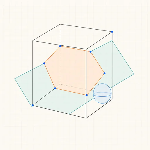
3D Geometry Board
Points, lines, planes, spheres and polyhedra on an orbiting camera — slice solids with planes, unfold nets, drop the Dandelin spheres into a cone and drag everything.
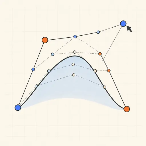
Bézier Curve Playground
Drag control points and watch De Casteljau’s algorithm construct a Bézier curve step by step.
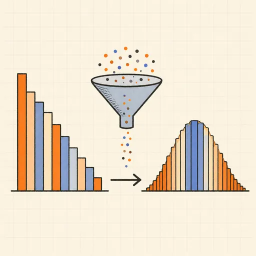
Central Limit Theorem Demo
Sample from any lopsided distribution and watch the averages pile up into a bell curve.
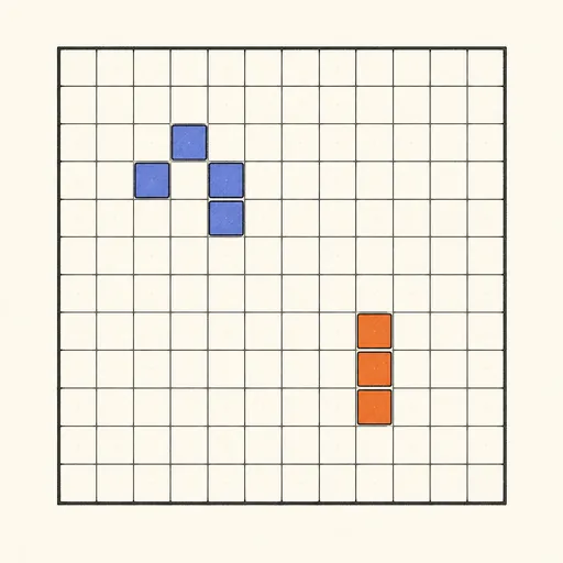
Conway’s Game of Life
Paint cells and watch Conway’s cellular automaton breed gliders, guns and oscillators.
Dynamic Geometry Board
Construct with points, lines, circles and transformations, then drag anything — the construction stays true, and a checker tells you which relations are theorems.
Fantasy Map Generator
Roll a seed and get a continent: coastlines, mountains, rivers, biomes and named towns, ready for your campaign.