Reaction–Diffusion Patterns, Explained
Read this and you will understand how two spreading, reacting chemicals turn a blank grid into spots, stripes and coral, why sliding two numbers switches between them, and how to reproduce the demo run number by number.
What the model is, and one example to hold onto
The Gray–Scott model tracks two chemicals on a grid. Call their concentrations u and v, each a number between 0 and 1 in every cell. Chemical u is supplied everywhere. Chemical v eats u and copies itself in the process, the reaction U + 2V -> 3V. Both chemicals also diffuse, spreading toward neighbors, with u spreading about twice as fast as v.
That is all. Yet start from a small square of v in a sea of u and, at the right rates, the square swells, pinches in the middle, and splits into two blobs. Each blob splits again. The grid fills with dividing spots that look like cells under a microscope. Nothing in the rules says "divide". The splitting is what the equations do on their own.
When this model is the right tool, and when it is not
Reach for Gray–Scott when you want to see how local rules build global patterns without any blueprint. It is a clean demonstration of Turing's 1952 idea that diffusion, usually a smoothing force, can instead create structure when it feeds a reaction. It is also a fair sketch of real skin-pattern chemistry, coral surfaces and some catalytic reactions.
Do not read it as a literal picture of any one organism. Real fish pigment involves many genes and cell types, not two chemicals. The model reproduces the look of spots and stripes, not their biochemistry. Treat the match as a strong hint that a Turing mechanism could be at work, not as proof that it is.
For a different self-organizing chemistry, the Belousov–Zhabotinsky Reaction oscillates in time and throws off rotating spiral waves. Gray–Scott, by contrast, usually settles into a pattern that is fixed in space.
The two equations and what each term does
The state changes in time by these rules, one for each chemical:
Here u and v are the two concentrations. The symbol \nabla^2 is the Laplacian, which on a grid just measures how much a cell sits below its neighbors' average, so D_u \nabla^2 u and D_v \nabla^2 v are diffusion. The diffusion rates are typically D_u = 0.16 and D_v = 0.08, the factor-of-two difference that makes patterns possible.
The term u v^2 is the reaction. It removes u and adds the same amount of v, and it grows fastest where v is already present, which is what makes it autocatalytic. The feed term f(1-u) tops u back up toward 1 at feed rate f. The removal term -(f+k)v drains v at the combined feed-plus-kill rate. Only f and k change from one pattern to the next.
A worked example that reproduces the demo
The demo starts from the field defaults: feed f = 0.037, kill k = 0.06, diffusion D_u = 0.16, D_v = 0.08, and a time step \Delta t = 1. Those rates sit in the "mitosis" regime, the self-replicating spots. Take one interior cell that currently holds u = 0.50 and v = 0.25, and suppose its four edge neighbors average u = 0.55 and v = 0.20.
One update step by hand
- Laplacian of u: neighbor average minus center,
0.55 - 0.50 = 0.05. Diffusion of u is 0.16 \times 0.05 = 0.008. - Laplacian of v:
0.20 - 0.25 = -0.05. Diffusion of v is 0.08 \times (-0.05) = -0.004. - Reaction term u v^2 = 0.50 \times 0.25^2 = 0.50 \times 0.0625 = 0.03125.
- Feed term f(1-u) = 0.037 \times 0.50 = 0.0185. Removal factor f+k = 0.097, so the v drain is 0.097 \times 0.25 = 0.02425.
- Change in u:
0.008 - 0.03125 + 0.0185 = -0.00475. New u = 0.50 - 0.00475 = 0.49525. - Change in v:
-0.004 + 0.03125 - 0.02425 = 0.003. New v = 0.25 + 0.003 = 0.25300.
In one step v rose by 0.003 and u fell by about 0.0048. The reaction is winning here, so this cell is filling with v. Repeat this arithmetic on every cell, thousands of times, and the spot pattern emerges. The tool does exactly this loop.
How feed and kill select the pattern
The whole zoo lives in a small window of the f–k plane, roughly f from 0.01 to 0.10 and k from 0.04 to 0.07. Pearson catalogued about a dozen regimes there in 1993. Small moves cross sharp borders. The table below gives rates that land you in each named preset.
| Pattern | Feed f | Kill k | What you see |
|---|---|---|---|
| Mitosis | 0.0367 | 0.0649 | Spots that split in two |
| Coral | 0.0545 | 0.062 | Branching growing tips |
| Spots | 0.03 | 0.062 | Stable dots, no splitting |
| Zebra stripes | 0.026 | 0.051 | Labyrinth of stripes |
| Worms | 0.058 | 0.065 | Wandering finite segments |
| Waves | 0.014 | 0.045 | Travelling fronts |
Notice how close mitosis and spots sit: same-ish kill, feed differing by only 0.007. That tiny gap is the difference between spots that divide forever and spots that freeze. The border is not gentle. This is why the parameter plane rewards slow, small slider moves.
What the field is telling you
The palette maps v concentration to color: navy where v is near 0, teal in the middle, cream where v is high. So cream regions are where the autocatalytic reaction is running hot, and navy is nearly pure fed-in u.
Watch how a pattern responds when you paint fresh v with the brush. In a stable regime the disturbance heals and the old pattern returns. In mitosis a new blob starts its own chain of divisions. In the labyrinth a fresh stroke reroutes nearby stripes. That healing-versus-invading response is the honest test of which regime you are in, more reliable than the still image.
Try the parameter plane yourself
The one thing a still picture cannot show is how the pattern reorganizes as you cross a border. Move the two rates and watch the regime flip.
Common mistakes
The errors below are the ones that waste the most time.
- Equal diffusion rates
- Set D_u = D_v and no pattern forms. The whole Turing mechanism needs the activator-ish and inhibitor-ish species to spread at different speeds. The standard 2-to-1 ratio is not decoration.
- Too large a time step
- Push \Delta t up to chase speed and the numbers explode into noise. The explicit scheme is only stable when the diffusion step per update stays small, roughly D_u \Delta t \le 0.5 in grid units.
- Reading a snapshot too early
- Early frames of almost every regime look like expanding blobs. Wait until the total v curve flattens (near step 1000 in the chart above) before naming the pattern.
- Confusing feed and kill
- Raising kill removes more v, thinning the pattern; raising feed supplies more u, feeding growth. Nudging the wrong one sends you across the wrong border.
A field that goes uniformly navy or uniformly cream is not a pattern, it is a failure. Uniform navy means v died out (kill too high, feed too low). Uniform cream means the reaction ran away. Step back toward a preset and change one rate at a time.
Related tools on this site
If self-organizing systems interest you, three neighbors on this site push the idea in other directions. The Crystal Growth Simulator builds branching fractals from random-walking particles, a different route to coral-like shapes. The Molecular Dynamics: Phases of Matter tool shows order emerging from moving atoms rather than reacting chemicals. The Flame Simulator lets you shape a reacting, diffusing fire with fuel and cooling controls.
Frequently asked questions
Why does U diffuse twice as fast as V?
The speed difference is what lets diffusion create structure instead of erasing it. A fast-spreading depleter and a slower-spreading grower set up the local imbalance that Turing predicted. Make the two rates equal and you get a flat, boring field.
Are these real chemicals?
Gray and Scott based the equations on a real cubic-autocatalytic reaction in a stirred tank. The two-dimensional patterns you see are a mathematical extension of that chemistry, matched later by experiments. So the model is chemically motivated but idealized, not a photograph of a specific reaction.
Why do the spots split in the mitosis regime?
A blob of v grows by consuming u at its edge, where fresh u arrives by diffusion. Its center starves because u cannot reach it fast enough, v collapses there, and the blob pinches into two. Each new blob repeats the cycle. It is starvation geometry, not a division program.
How long until a pattern settles?
In the worked demo the total v curve is still rising steeply at step 200 and only flattens near step 1000. Expect several hundred to a couple of thousand steps before the texture is trustworthy, more for large grids.
Can I get the same pattern to look different each run?
Yes. The rates fix the pattern type, but the random starting squares fix the exact placement. Reseed and you get a new labyrinth or a new arrangement of spots in the same regime. The statistics (spot size, stripe spacing) stay the same while the layout changes.
Related tools
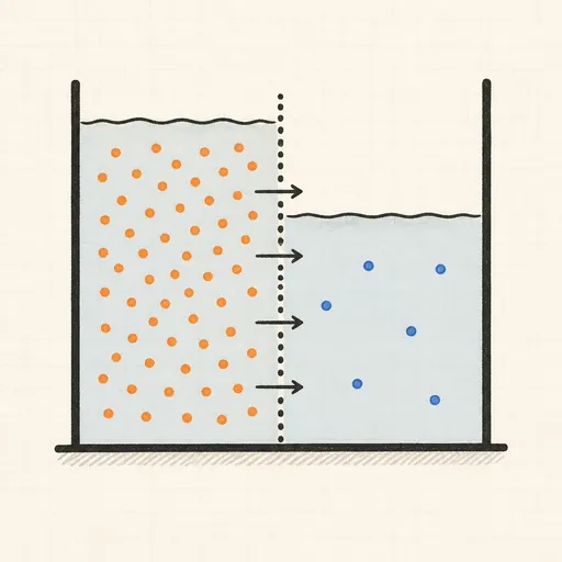
Diffusion & Osmosis
Split a tank with a semipermeable wall and watch particles diffuse and water flow to equalise concentration.
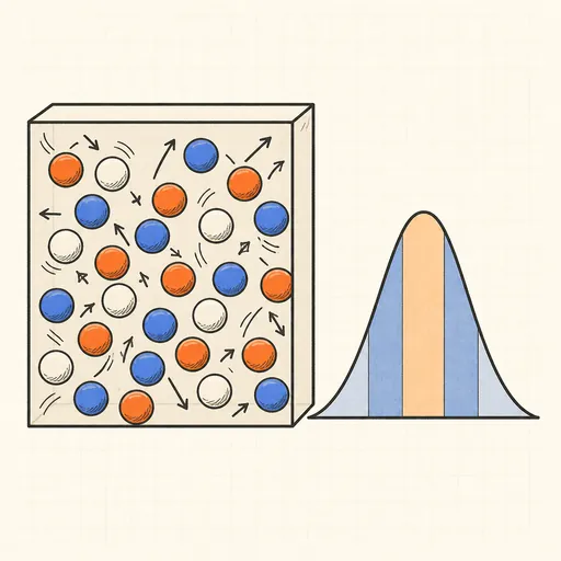
Ideal Gas & Maxwell–Boltzmann
Bounce hard-disc molecules in a box and watch their speeds settle into the Maxwell–Boltzmann distribution.
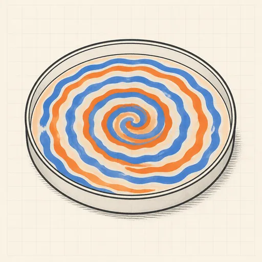
Belousov–Zhabotinsky Reaction
Watch an oscillating chemical medium organize itself into rotating spiral waves.
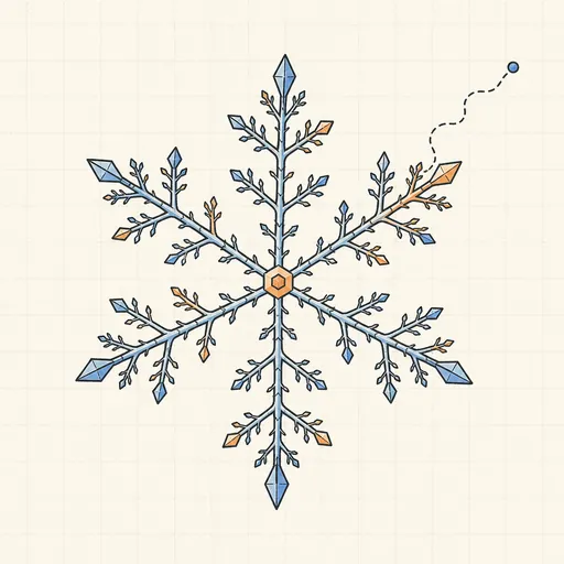
Crystal Growth Simulator
Grow branching fractal crystals one wandering particle at a time with diffusion-limited aggregation.

Flame Simulator
Paint fire and shape a living flame with fuel, cooling, wind and turbulence.
Ising Model Ferromagnet
Flip a grid of spins at any temperature and watch magnetic domains freeze in or melt at the critical point.