Percolation, Explained
Read this and you will know why a grid of independent coin flips suddenly starts to conduct at one sharp probability, how to estimate that threshold yourself, and how to tell a spanning cluster from noise.
What percolation is, with one hook
Take a square grid. Visit every cell and, independently, mark it open with probability p or closed with probability 1-p. Open cells that touch edge to edge form clusters. The question percolation asks is blunt: does any single cluster reach from the top row to the bottom row?
At p = 0.50 on a large square grid the answer is almost always no. The open cells cover half the grid, yet the largest connected blob stops well short of spanning. Nudge p up to 0.62 and the answer flips to almost always yes. A single cluster now stretches across the whole grid. The change happens in a window only a few hundredths of a unit wide, and it gets sharper as the grid grows.
That is the hook. Nothing coordinates the cells. Each is an isolated coin flip. Still, connectivity appears as a threshold effect, not a gradual slope. This is the defining feature of percolation and the reason it shows up wherever something spreads through a random medium.
When to reach for this model, and when not
Percolation is the right first model when three things hold: the medium is roughly random, the units are either passable or blocked, and what you care about is global connectivity rather than fine timing. Current through a sheet with random broken contacts fits. Water seeping through soil with random pores fits. A rumour crossing a social graph where each tie either transmits or does not fits.
The tool here uses site percolation: cells (sites) are open or closed. A close cousin, bond percolation, opens the links between cells instead. The two share the same abrupt-threshold story but land at different critical values, so do not mix up which one your problem is.
Percolation is a static, geometric model. It tells you whether a path exists, not how fast anything moves along it or how the pattern changes in time. If your real question is about dynamics (a wave that oscillates, a front that advances at some speed), a purely geometric threshold will mislead you.
Do not use it when the units interact. Real forest fires reshape the fuel ahead of them, real diseases confer immunity, real conductors heat up. Basic percolation assumes independent, fixed cells. It gives you the connectivity backbone; it does not give you the feedback.
The threshold and the order parameter
Two numbers carry the whole story. The first is the critical probability p_c, the value of p at which a spanning cluster first appears in the infinite-grid limit. For site percolation on a square lattice it has no closed form, but numerical work pins it at:
Here p is the open-cell probability and p_c is the special value that separates the two regimes. Below it, no spanning; above it, spanning becomes near-certain on a large grid.
The second number is the percolation probability P_\infty(p), the fraction of the grid taken up by the single largest cluster once the grid is large. It behaves like an order parameter in physics: flat at zero below the threshold, then rising from zero above it along a power law.
In this expression \beta is a critical exponent. For two-dimensional percolation \beta = 5/36 \approx 0.139. The small exponent matters: it makes the giant cluster rise steeply just above p_c. Plug in p - p_c = 0.01 and you get 0.01^{0.139} \approx 0.523, so even a one-percent overshoot already fills about half the grid in the ideal limit.
The exponent \beta = 5/36 is universal: it is the same for site and bond percolation, for square, triangular and honeycomb lattices, even though p_c differs for each. Only the dimension of space fixes the exponent, not the lattice details.
A worked example on a small grid
The demo fills the grid at the tool's default settings. Because a real finite grid does not have a razor-sharp threshold, work through what you should expect at several values of p, then check the demo against it.
Estimating the spanning probability by sweeping p
Consider a large square grid and sweep p from 0.50 to 0.70. For each p, ask over many random fills: what fraction of fills produce a top-to-bottom spanning cluster? Call that the spanning probability. On an infinite grid it is a step at 0.5927. On a finite grid it is a smooth S-curve centred there.
- At
p = 0.50, open cells cover half the grid but sit in scattered clumps. Spanning probability is near0.02. You will rarely see a spanning cluster. - At
p = 0.55, clusters merge into larger islands. Spanning probability climbs to roughly0.18. Some fills span, most do not. - At
p = 0.5927, you are on the threshold. Spanning probability is about0.50: a coin flip on any given fill. - At
p = 0.63, one cluster usually dominates. Spanning probability is around0.86. - At
p = 0.68, spanning is nearly guaranteed at about0.99. The grid conducts on almost every fill.
The lesson is that the transition is centred at p_c but has width. That width shrinks as the grid grows. Double the side length and the S-curve steepens; push toward an infinite grid and it becomes the vertical step the theory predicts.
Reading and interpreting the coloured clusters
The tool floods each connected cluster in its own colour and highlights any cluster that spans. Three things are worth reading off the picture.
- Largest cluster size
- Below p_c the biggest cluster is small compared with the grid and grows only slowly with grid size. Above p_c it takes a finite fraction of the whole and grows in step with the grid area.
- Cluster size distribution
- Exactly at p_c clusters come in every size, following a power law. You see a few large clusters, more medium ones, and many tiny ones, with no single scale standing out.
- Spanning flag
- The one binary readout: is there a path from top to bottom. On a finite grid this flickers on and off near p_c because it depends on the exact random fill.
Because a finite grid blurs the threshold, judge the transition location by where spanning happens about half the time, not by a single lucky fill. Run the same p several times and count.
Common mistakes when using the model
The errors below are the ones that most often make people misread what they see.
- Reading one fill as the truth. Near p_c a single grid may span or not by chance. At
p = 0.5927your odds of spanning are about even, so one run says nothing. Average over many. - Confusing coverage with connectivity. At
p = 0.55more than half the cells are open, yet the grid usually does not span. Coverage of half is not the same as a connected path across. - Expecting the finite-grid threshold to equal 0.5927 exactly. The clean value is the infinite-grid limit. A small grid spans, on average, at a slightly different value and with a wide transition. Only as the grid grows does the crossover tighten onto
0.5927. - Mixing site and bond percolation. Bond percolation on the square lattice has p_c = 0.5 exactly, not
0.5927. Using the wrong threshold for your problem shifts your prediction by nearly a tenth. - Treating diagonal touches as connections. This tool connects cells that share an edge, not a corner. Allowing diagonal links changes the lattice and lowers p_c. Be clear which rule your real system follows.
Related simulations to explore next
Percolation is the geometric skeleton of many spreading and phase-change ideas on this site. A few neighbours make the connections concrete.
The sharp jump at p_c is a phase transition, and the closest cousin is the Ising Model Ferromagnet, where magnetic order appears at a critical temperature the same abrupt way. For a spreading process with real dynamics rather than static geometry, the Flame Simulator shows how a front moves once a path exists. If you want to watch structure grow from randomness rather than merely connect, the Crystal Growth Simulator builds branching clusters one wandering particle at a time. And for the independent-particle bookkeeping that underlies statistical models generally, the Ideal Gas & Maxwell-Boltzmann tool shows a distribution emerging from many uncoordinated events.
Frequently asked questions
Why is the percolation threshold near 0.5927 and not 0.5?
The value 0.5927 is specific to site percolation on a square lattice with edge-only connections. It has no simple formula and comes from careful numerical simulation. The rounder value 0.5 belongs to bond percolation on the same lattice, which is a different rule. Change the lattice or the rule and the threshold changes.
Does the threshold depend on the grid size?
The location converges to 0.5927 as the grid grows, but the sharpness depends strongly on size. On a 20 by 20 grid the transition from rarely-spanning to almost-always-spanning spans a window about 0.14 wide. On a 200 by 200 grid that window shrinks to roughly 0.04. Bigger grids give a crisper answer.
What does it mean that the grid "conducts"?
Picture open cells as conducting material and closed cells as insulator. If a cluster spans top to bottom, current can flow across; the grid conducts. If no cluster spans, every path is broken somewhere and no current crosses. The spanning question and the conduction question are the same question.
Why does the giant cluster appear so suddenly?
Just below p_c, adding a few open cells mostly grows separate small clusters. Just above it, those same additions splice medium clusters into one another, and the merged cluster then absorbs its neighbours in a chain. The small exponent \beta = 5/36 captures this: the largest-cluster fraction rises like (p-p_c)^{0.139}, which is nearly vertical right at the threshold.
Can percolation predict a real forest fire or epidemic?
It gives the connectivity part and nothing else. It can tell you whether a fully susceptible, randomly arranged medium admits a spanning path, and it warns you that the change is a threshold rather than a slope. It cannot handle immunity, wind, regrowth, or timing, all of which need dynamic models on top of the static skeleton.
Related tools
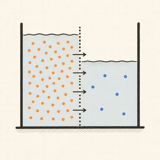
Diffusion & Osmosis
Split a tank with a semipermeable wall and watch particles diffuse and water flow to equalise concentration.
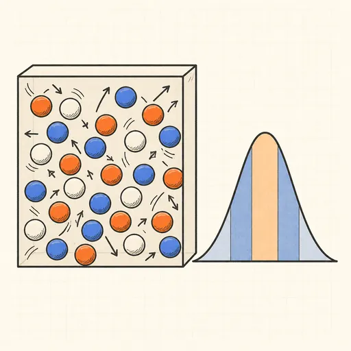
Ideal Gas & Maxwell–Boltzmann
Bounce hard-disc molecules in a box and watch their speeds settle into the Maxwell–Boltzmann distribution.
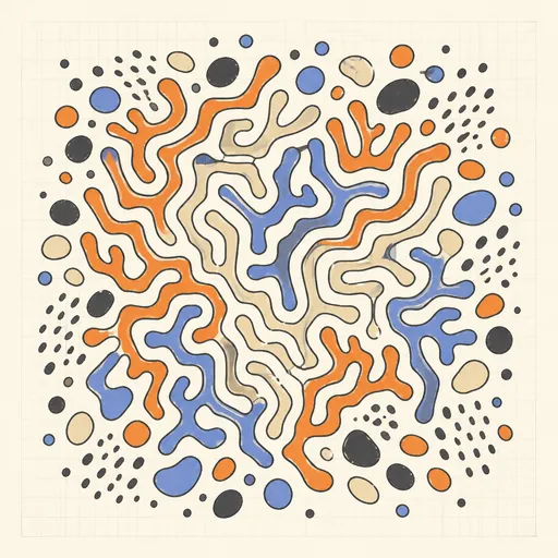
Reaction–Diffusion Patterns
Grow coral, spots and zebra stripes from two virtual chemicals with the Gray–Scott model.
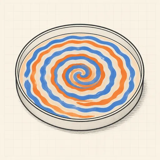
Belousov–Zhabotinsky Reaction
Watch an oscillating chemical medium organize itself into rotating spiral waves.
Crystal Growth Simulator
Grow branching fractal crystals one wandering particle at a time with diffusion-limited aggregation.
Flame Simulator
Paint fire and shape a living flame with fuel, cooling, wind and turbulence.