The Belousov–Zhabotinsky Reaction, Explained
After reading this you can explain why a chemical medium oscillates instead of settling, derive the three-species cyclic update this simulation runs, and predict how the reaction rates change the size and shape of the spiral waves.
What it is, and the beaker that would not settle down
Most chemistry runs downhill to equilibrium and stays there. Mix vinegar and baking soda, wait, and nothing else happens. The Belousov–Zhabotinsky reaction breaks that expectation. In a shallow dish the mixture flips colour on a clock: blue, then orange, then blue again, over and over for many minutes. Leave it still and the colour changes spread as expanding rings and rotating spirals, like ripples that keep coming from nowhere.
That behaviour looks like it violates the second law of thermodynamics, which is exactly why journals rejected Belousov's paper in the 1950s. It does not. The reaction is far from equilibrium and burns through a store of chemical fuel (bromate and malonic acid) while it oscillates. The colour swing comes from a catalyst, ferroin, that switches between two oxidation states. The system is still marching toward equilibrium, but it does so by circling rather than by sliding straight down.
This simulation does not track real molecules. It runs a compact cyclic model that reproduces the same waves. Three abstract concentrations a, b and c live on every cell of a grid. Each step mixes each cell with its neighbours, then lets the three quantities feed on each other in a loop. Start from random noise and within a few seconds the grid organizes into target rings and spirals.
When this model helps, and when it misleads
Use this simulation to build intuition about excitable media: systems that sit quietly until a small kick pushes them over a threshold, fire a large response, then reset and wait. The BZ dish is the textbook example, but the same spiral waves appear in heart muscle and in slime-mould colonies. If you want to see how a local disturbance becomes a travelling wave, and how waves annihilate when they collide, this is a faithful cartoon.
Do not read chemical rate constants off the sliders. The \alpha, \beta and \gamma values here are dimensionless knobs in a cyclic toy model, not the rate coefficients of the Oregonator mechanism. The model captures the qualitative behaviour (oscillation, wavelength, spiral formation) and gets the numbers wrong on purpose, because getting them right would require the full reaction network and stiff differential equations.
If you want pattern formation driven by two diffusing chemicals rather than a three-species cycle, see the Reaction–Diffusion Patterns tool, which runs the Gray–Scott model and grows spots and stripes instead of rotating spirals.
The update rule and the intuition behind it
Each cell holds three numbers, all clamped to the range 0 to 1. Write them a, b, c. One time step has two stages.
Stage 1: diffusion. Replace each concentration by the average over the cell and its eight neighbours. This is the stirring. Diffusion alone smooths everything toward a flat grey and would kill any pattern on its own.
Stage 2: reaction. Apply the cyclic feeding rule. Using the averaged values, written with a bar, the next values are:
Here a' is the new value of the first species. The term \alpha \bar{b} makes a grow in proportion to how much b is present nearby: a eats b. The term \gamma \bar{c} makes a shrink where c is present: c eats a. The other two species follow the same pattern, rotated:
Read the three together and the loop is clear: a beats b, b beats c, c beats a. That is rock-paper-scissors. No species can win outright, so no cell settles. Instead each cell cycles through dominance by a, then b, then c. Diffusion couples neighbours so that neighbouring cells fall slightly out of phase, and a phase gradient is exactly what a travelling wave is. After each reaction stage every value is clamped back into [0, 1]. The colour you see maps this state to a ferroin-style blue, orange and white banding.
Worked example: one cell over three steps
Run the model with the defaults \alpha = 1, \beta = 1, \gamma = 1. To follow the reaction alone, imagine a small patch where all neighbours already share one cell's values, so the averages equal the cell itself: \bar{a} = a, and so on. Start slightly away from balance: a = 0.6, b = 0.3, c = 0.1.
- Step 1. a' = 0.6 + 0.6(0.3 - 0.1) = 0.6 + 0.12 = 0.72. b' = 0.3 + 0.3(0.1 - 0.6) = 0.3 - 0.15 = 0.15. c' = 0.1 + 0.1(0.6 - 0.3) = 0.1 + 0.03 = 0.13.
- Step 2. Feed
(0.72, 0.15, 0.13)back in. a' = 0.72 + 0.72(0.15 - 0.13) = 0.7344. b' = 0.15 + 0.15(0.13 - 0.72) = 0.06150. c' = 0.13 + 0.13(0.72 - 0.15) = 0.2041. - Step 3. Feed
(0.7344, 0.06150, 0.2041)back in. a' = 0.7344 + 0.7344(0.06150 - 0.2041) = 0.6297. b' keeps falling as a dominates it, and c keeps climbing because a is large.
Watch the ranking. At the start a \gt b \gt c. By step 3, c has overtaken b and is chasing a down. Keep iterating and c will eventually overtake a, then b will recover and overtake c, and the cycle repeats. A single isolated cell oscillates. Coupling many such cells with the diffusion stage is what turns the oscillation into a spatial wave.
a in a single well-mixed cell. It settles into a steady oscillation with a period near 14 steps rather than decaying to a fixed value.Explore the rates yourself
Reading the patterns on the grid
Once the full grid runs, three structures appear. Learn to name them.
- Target rings
- Concentric circles expanding from a point. They form around a pacemaker: a spot that happens to cycle slightly faster than its surroundings and keeps launching fresh waves outward.
- Spiral waves
- Curved arms rotating around a fixed centre. A spiral appears when a wave front is broken, for example when two rings collide or when you inject excitation into a partly recovered region. The free end curls and becomes a self-sustaining rotor.
- Wave collisions
- When two fronts meet they do not pass through each other. Each front leaves behind a region that is still resetting and cannot fire yet, so the fronts annihilate. This is why the dish never fills solid: waves keep eating each other.
Wavelength is the distance between successive fronts. Faster reaction rates cycle each cell more quickly, so a front spends less time in each place and the spacing between fronts shrinks. Expect higher \alpha, \beta and \gamma to give tighter, busier spirals, and lower values to give broad, slow rings. The diffusion stage sets the front speed: with the fixed nine-cell averaging here, a front advances on the order of one cell per step.
Common mistakes when interpreting the simulation
Do not expect a stable final picture. This is not a tool that converges. If you wait for the pattern to stop changing, you will wait forever, because a non-converging oscillation is the whole point. Judge it by the character of the motion, not by a resting state.
A second mistake is starting from a perfectly uniform field and expecting waves. If every cell holds identical values, the diffusion average changes nothing and every cell oscillates in lockstep. The whole dish then flashes as one block, with no spatial structure. Waves need phase differences between neighbours, which is why the simulation seeds from random noise and why clicking to inject excitation kicks a region out of phase.
A third mistake is treating the three sliders as independent tuning of three colours. They are the three arms of one cycle. Push \alpha far above \beta and \gamma and you unbalance the loop: one species tends to dominate longer, the oscillation grows lopsided, and at extreme settings the clamping to [0, 1] can freeze regions. Balanced rates give the cleanest spirals.
Related simulations on this site
The BZ dish is one member of a family of local-rule models that build large structure from simple neighbour interactions. If spiral waves interest you, these neighbours are worth a look.
- The Reaction–Diffusion Patterns tool uses two chemicals and the Gray–Scott equations to grow spots, stripes and coral-like mazes. It is the steady-pattern cousin of this oscillating one.
- The Crystal Growth Simulator grows branching fractals by diffusion-limited aggregation, where random walkers stick on contact. It shows a different way diffusion shapes structure.
- The Molecular Dynamics: Phases of Matter tool tracks individual particles under Lennard-Jones forces and shows gas, liquid and crystal. It is the bottom-up counterpart to these continuum grids.
- The Flame Simulator is another excitable, advecting medium, tuned for fuel and turbulence rather than chemical cycling.
Frequently asked questions
Why does the real BZ reaction change colour?
The catalyst ferroin switches between a reduced state (red or orange) and an oxidized state (blue) as the concentration of bromide ions rises and falls. The oscillation in bromide, driven by the bromate-malonic-acid network, drives the colour with it. The simulation imitates the colour band without simulating the actual ions.
Is the oscillation breaking the second law of thermodynamics?
No. The mixture is far from equilibrium and consumes bromate and malonic acid the whole time. Total free energy falls steadily even while the visible colour oscillates. The system is spending fuel to circle toward equilibrium rather than sliding straight there. Belousov's reviewers got this wrong in the 1950s.
Why do spirals form instead of simple rings?
Rings come from an intact pacemaker sending out complete circular fronts. A spiral needs a broken front. When one front is cut, for example by colliding with another wave or with a region that is still recovering, the free tip curls around the point it cannot cross. That curling tip circulates and pumps out a spiral arm indefinitely.
What do the three sliders actually change?
They set the three rates in the cyclic feeding rule. Raising all three together speeds up each cell's cycle, which shortens the period (near 14 steps at the defaults) and tightens the wavelength. Making one much larger than the others unbalances the rock-paper-scissors loop and distorts the spirals. They are not per-colour brightness controls.
Does this simulation match a real dish quantitatively?
No. It reproduces the qualitative behaviour: oscillation, target rings, rotating spirals, front annihilation. The slider values are dimensionless and do not correspond to measured rate constants. For quantitative BZ work you would integrate the Oregonator differential equations with real coefficients.
Related tools
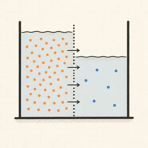
Diffusion & Osmosis
Split a tank with a semipermeable wall and watch particles diffuse and water flow to equalise concentration.
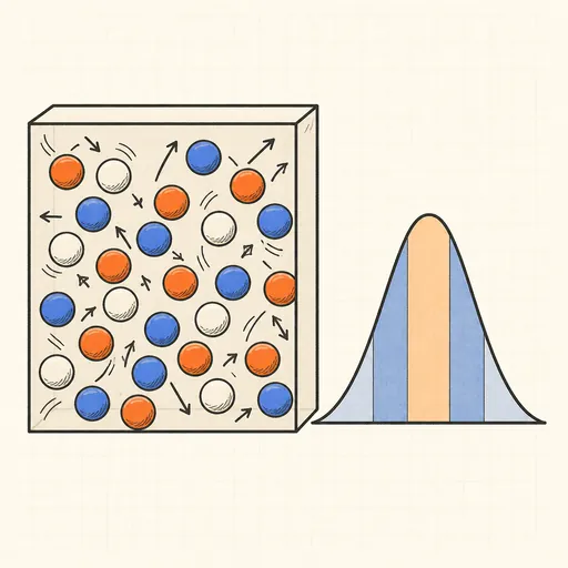
Ideal Gas & Maxwell–Boltzmann
Bounce hard-disc molecules in a box and watch their speeds settle into the Maxwell–Boltzmann distribution.
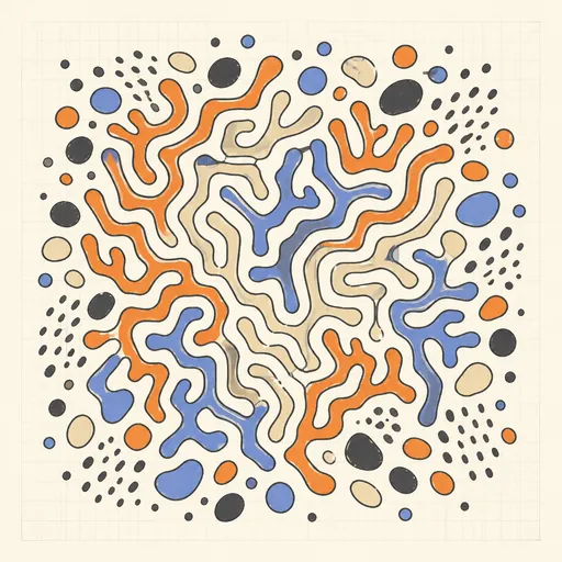
Reaction–Diffusion Patterns
Grow coral, spots and zebra stripes from two virtual chemicals with the Gray–Scott model.
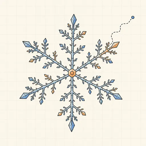
Crystal Growth Simulator
Grow branching fractal crystals one wandering particle at a time with diffusion-limited aggregation.
Flame Simulator
Paint fire and shape a living flame with fuel, cooling, wind and turbulence.
Ising Model Ferromagnet
Flip a grid of spins at any temperature and watch magnetic domains freeze in or melt at the critical point.