Monte Carlo Methods, Explained
After reading this you will know how random sampling turns a hard question into an average, how to predict the error before you run anything, and how to read the two charts that every panel of the playground draws.
What Monte Carlo actually does
Monte Carlo means answering a question by sampling at random and averaging. That is the whole idea. If you can phrase your question as "what is the average of some random quantity," you can estimate it by drawing samples and taking their mean. You do not need a formula for the answer. You only need a way to draw fair samples.
Start with the classic hook: estimating \pi with darts. Draw a square from -1 to 1 on each axis, and inscribe the unit circle inside it. The square has area 4. The circle has area \pi. Throw darts uniformly at the square. The fraction landing inside the circle should be about \pi / 4 \approx 0.7854. Multiply that fraction by 4 and you have an estimate of \pi.
Throw 1000 darts and maybe 786 land inside. Your estimate is 4 × 0.786 = 3.144. The true value is 3.14159. Not bad for counting dots. Throw more darts and the estimate tightens. Nothing here knows any geometry beyond "is this point closer than 1 to the origin." The randomness does the work.
When to reach for it, and when not
Monte Carlo shines when the problem has many dimensions or no closed form. Pricing a retirement portfolio over 30 years of correlated returns has no tidy formula. A grid of scenarios in 30 dimensions is hopeless: even 10 points per axis is 10^{30} cells. Random sampling ignores dimension. It converges at the same rate whether the problem lives in 2 dimensions or 200.
Skip Monte Carlo when a formula already exists. If you want the area of a circle, use \pi r^2. Sampling would only add noise to an exact answer. Also skip it when you cannot sample fairly. A biased random generator gives a confident wrong number, and the charts will look just as smooth while lying to you.
The playground's game mode uses the same averaging idea in a different costume. Monte Carlo tree search plays out random games to the end, then averages the wins. A move that wins 640 of 1000 random playouts scores 0.64, and the search spends more playouts on the promising branches.
The one formula behind every panel
Let X_1, X_2, \ldots, X_N be independent samples of some random quantity with true mean \mu and standard deviation \sigma. The estimate is the sample average:
Here \hat{\mu}_N is your running estimate after N samples, and each X_i is one sample: 1 if a dart lands in the circle and 0 if not, or one simulated final portfolio value, or 1 for a game won. The law of large numbers guarantees \hat{\mu}_N \to \mu as N grows.
The error is where the real insight lives. The standard error of the estimate is:
The symbol \sigma is the spread of a single sample, and N is how many you drew. The error falls like 1/\sqrt{N}. That is the central fact of the whole method. To halve the error you must quadruple the samples, because \sqrt{4} = 2. To cut the error by 10 you need 100 times the samples.
Worked example: estimating pi with the demo defaults
1000 darts on the unit square
Run the dart demo with its default of 1000 samples. Each dart is a point (x, y) with x and y drawn uniformly from -1 to 1. It counts as a hit when x^2 + y^2 \le 1.
- The expected hit fraction is the ratio of areas: \pi/4 \approx 0.7854.
- Over 1000 throws you expect about
785hits. Suppose a run gives 793. - The hit fraction is
793 / 1000 = 0.793. - The estimate of \pi is
4 × 0.793 = 3.172. - Predict the error. For a hit-or-miss estimator the per-sample \sigma of the scaled value is 4\sqrt{0.7854 \cdot 0.2146} \approx 1.643. Then \text{SE} = 1.643 / \sqrt{1000} \approx 0.0520.
So one run of 1000 darts should land within roughly 0.05 of 3.14159 about two thirds of the time. Your 3.172 sits 0.030 away, comfortably inside that band. Push to 100000 darts and the predicted error drops to 1.643/\sqrt{100000} \approx 0.0052, ten times smaller.
Reading the two charts
Every mode drives the same pair of charts. The first is the running estimate against N. Early on it lurches. By 10000 samples it hugs the true value. The lurches are not bugs. They are the finite-sample noise shrinking on schedule.
The second chart is the error on a log-log plot. Take logs of both sides of \text{SE} = \sigma / \sqrt{N}:
That is a straight line with slope -\tfrac{1}{2}. On the log-log axes your measured error should scatter around a line of that slope. If your points fall faster, you got lucky on this run. If they flatten out and stop falling, something is wrong: often a biased sampler, so the estimate converges to the wrong number and the error stalls at that gap.
Common mistakes
The most frequent error is expecting linear payoff from more samples. Going from 1000 to 2000 samples does not halve the error. It cuts it by a factor of \sqrt{2} \approx 1.41, only about 29 percent. Plan your compute budget around 1/\sqrt{N}, not 1/N.
The second mistake is trusting a smooth curve. A biased random source produces a confident estimate that converges to the wrong value. The Buffon's needle panel is a good teacher here: if you drop needles longer than the line spacing, the crossing probability formula changes, and naively applying the short-needle formula gives a wrong \pi that never corrects no matter how many needles you drop.
Correlated samples break the square-root law. If today's simulated market return depends on yesterday's and you treat the two as independent, your true error is larger than \sigma/\sqrt{N} and your confidence band is too narrow. The estimate will look tighter than it is.
A third trap in the retirement panel is confusing the average outcome with the risk. A portfolio can have a healthy mean final value while 1 path in 10 runs out of money. Read the tail of the distribution, not just the center. Monte Carlo hands you the whole spread of outcomes for free, so use it.
Related tools
Randomness building structure is a theme across this site. The Chaos Game jumps to random corners yet paints a fixed Sierpinski triangle, another case of order from noise. The Random Walk Explorer shares the exact 1/\sqrt{N} scaling: a drunkard's distance from the start grows like the square root of steps, the same law as Monte Carlo error.
For the deterministic-chaos side, the Logistic Map Bifurcation and the Lorenz Attractor show systems that look random but follow fixed rules. The Conway's Game of Life and Elementary Cellular Automata generate complex patterns from simple update rules, a useful contrast to sampling-based methods.
Frequently asked questions
Why does the error shrink as 1 over the square root of N?
The variance of an average of N independent samples is the single-sample variance divided by N. Taking the square root to get the standard deviation gives \sigma/\sqrt{N}. The 1/\sqrt{N} falls straight out of dividing variance by N.
How many samples do I need?
Solve \sigma/\sqrt{N} = e for your target error e, giving N = (\sigma/e)^2. For the pi darts with \sigma \approx 1.643, hitting an error of 0.01 needs N = (1.643/0.01)^2 \approx 27000 samples.
Is Monte Carlo better than a grid of evenly spaced points?
In one or two dimensions a grid usually wins. Monte Carlo overtakes grids in high dimensions because its 1/\sqrt{N} rate does not depend on dimension, while a grid's accuracy degrades as N^{-1/d} with dimension d. At d = 4 the two rates already match, and beyond that Monte Carlo pulls ahead.
Why does the game mode use UCB instead of pure random playouts?
Pure random playouts waste effort on obviously bad moves. UCB (upper confidence bound) balances trying the current best move against exploring uncertain ones, spending playouts where they change the verdict. It is the same averaging engine with a smarter allocation of samples.
Can I trust a Monte Carlo answer that looks converged?
Only if your sampler is unbiased and your samples are independent. A converged-looking curve from a biased source settles on the wrong number. Check convergence by running with different random seeds and confirming the estimates agree within their predicted error bands.
Related tools
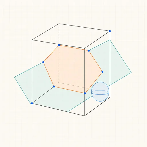
3D Geometry Board
Points, lines, planes, spheres and polyhedra on an orbiting camera — slice solids with planes, unfold nets, drop the Dandelin spheres into a cone and drag everything.
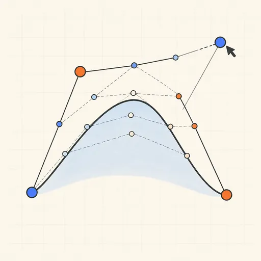
Bézier Curve Playground
Drag control points and watch De Casteljau’s algorithm construct a Bézier curve step by step.
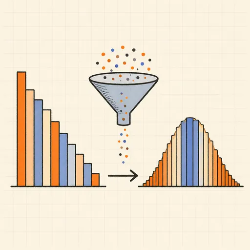
Central Limit Theorem Demo
Sample from any lopsided distribution and watch the averages pile up into a bell curve.
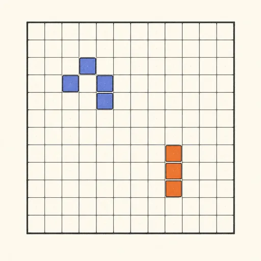
Conway’s Game of Life
Paint cells and watch Conway’s cellular automaton breed gliders, guns and oscillators.
Dynamic Geometry Board
Construct with points, lines, circles and transformations, then drag anything — the construction stays true, and a checker tells you which relations are theorems.

Fantasy Map Generator
Roll a seed and get a continent: coastlines, mountains, rivers, biomes and named towns, ready for your campaign.