The Law of Large Numbers, Explained
After reading this you can predict how fast a running average settles onto its expected value, put a number on the leftover wobble, and explain why the gambler's fallacy is wrong even though the average really does converge.
What the law of large numbers says
Roll a fair six-sided die once and you might get a 2. Roll it ten times and the average could be 3.1 or 4.4. Keep rolling into the thousands and the average locks onto 3.5 and stays there. That pinning-down is the law of large numbers: the average of many independent trials converges to the expected value.
The expected value of one fair die is the plain average of its faces. Add 1+2+3+4+5+6 = 21 and divide by 6 to get 3.5. No single roll can produce 3.5, yet the average of enough rolls will sit right on it. The simulator makes this visible: it plots the running mean as trials pile up and draws a shrinking band that shows how far off you should expect to be at each point.
The hook is that two different quantities behave in opposite ways at once. The average of heads settles toward 0.5. The count of heads minus tails does not settle at all; it keeps wandering, and typically grows. Both facts are true together, and confusing them is the source of a lot of bad betting.
When it applies and when it does not
The law needs three things. The trials must be independent, so one roll tells you nothing about the next. They must come from the same distribution, so the die does not change between rolls. And that distribution must have a finite expected value.
The finite-mean condition is not a technicality. The St. Petersburg paradox is a game whose expected payout is infinite, and its running average never settles: it keeps lurching upward with every rare jackpot. Feed that into a convergence plot and you see a staircase, not a flat line. The law of large numbers has nothing to say there.
Independence is the assumption most often broken in the real world. Card draws without replacement, weather on consecutive days, and repeated measurements on a warming instrument are all correlated. The running average may still move, but the 1/\sqrt{n} shrinkage below can be badly wrong when trials are linked.
The formula and the intuition behind it
Write the outcome of trial i as X_i, and let the running mean after n trials be:
Here \bar{X}_n is the average of the first n results. The weak law says that for any tolerance \varepsilon \gt 0, the probability that \bar{X}_n lands more than \varepsilon away from the true mean \mu goes to zero as n grows.
That tells you the average gets close, but not how fast. The speed comes from the variance. If one trial has variance \sigma^2, then the running mean has variance \sigma^2/n, so its typical spread is the square root of that:
\sigma is the standard deviation of a single trial. The key fact is the \sqrt{n} in the denominator. To halve the typical error you need four times as many trials. To cut it to a tenth you need a hundred times as many. Convergence is real but slow.
For a fair die, \sigma^2 = 35/12 \approx 2.917, so \sigma \approx 1.708. After 100 rolls the running mean typically sits within 1.708/\sqrt{100} = 0.171 of 3.5. After 10,000 rolls that band is 1.708/100 = 0.0171, ten times tighter for a hundred times the work.
Reproducing the demo: rolling one die
A fair die, band by band
Load the tool with its defaults (a single fair six-sided die) and press the demo button. The expected value is 3.5. Here is what the shrinking band predicts at four checkpoints, using \sigma \approx 1.708.
- At
n = 10: band width 1.708/\sqrt{10} = 0.540. Expect the running mean somewhere in[2.96, 4.04]. - At
n = 100: band 1.708/\sqrt{100} = 0.171, range[3.33, 3.67]. - At
n = 1000: band 1.708/\sqrt{1000} = 0.0540, range[3.446, 3.554]. - At
n = 10000: band 0.0171, range[3.483, 3.517].
These are one-standard-deviation bands, so about 68% of runs stay inside them and roughly a third stray outside at any given point. That is expected, not a bug. If every run hugged the line perfectly, the randomness would be gone.
The average settles, the count does not
Switch to the coin. Expected value of heads is 0.5. Watch two lines at once and you meet the sharpest lesson in the whole subject.
The running proportion of heads converges to 0.5. Its typical distance from 0.5 after n flips is 0.5/\sqrt{n}, using \sigma = 0.5 for a fair coin. After 10,000 flips that is 0.005, so the proportion is pinned near half.
Now track heads minus tails. This is a random walk, and its typical size grows like \sqrt{n}. After 10,000 flips the count is typically about \sqrt{10000} = 100 away from zero, and after a million flips about 1000 away. The gap is not shrinking. It is widening.
Both statements hold together because the proportion is the count divided by n. A gap of size \sqrt{n} divided by n is 1/\sqrt{n}, which shrinks. The count wanders off while the average tames it by dividing by a bigger and bigger number. For the same wandering-count idea on its own, see the Random Walk Explorer.
Reading your own results
When you run the tool, judge convergence against the band, not against a fixed target. Three habits keep you honest.
First, expect roughly one run in three to poke outside the one-sigma band at any snapshot. A single excursion is not a broken simulation. Second, remember the horizontal axis usually spaces trials evenly, so the eye-catching stabilization in the last stretch is partly a scale illusion: the band at n = 9000 and n = 10000 differ by almost nothing. Third, if you use a custom distribution, compute its mean and variance first so you know what the plot should approach.
- Expected value \mu
- The probability-weighted average of outcomes. For a fair die,
3.5. - Running mean \bar{X}_n
- The average of the first
noutcomes so far. Updated after each trial. - Standard error
- The typical distance of the running mean from \mu, equal to \sigma/\sqrt{n}.
- Weak law
- The average is very likely close to \mu for large
n, not certain to equal it.
Common mistakes
The biggest is the gambler's fallacy. After eight heads in a row, tails is not due. The coin has no memory. The proportion recovers toward 0.5 not by reversing the streak but by drowning it: those eight extra heads become a smaller and smaller slice of the total as flips accumulate. At n = 8 they are the whole story; at n = 10000 they move the proportion by 8/10000 = 0.0008.
Test this yourself: flip a coin to a long streak, then keep going and watch the proportion. It slides toward 0.5 without any compensating run of tails. The streak is not undone, it is diluted.
Two more traps. Confusing the law of large numbers with the central limit theorem: the first says the average converges, the second describes the bell-shaped distribution of that average around the mean. See the Central Limit Theorem Demo for the second. And forgetting that convergence is slow. Estimating a proportion to within 0.001 for a coin needs about (0.5/0.001)^2 = 250{,}000 flips. Precision costs sample size quadratically.
Related tools
The same convergence idea drives estimation by sampling. The Monte Carlo Playground and Buffon's Needle both estimate numbers like \pi by averaging many random trials, and both slow down at the same 1/\sqrt{n} rate. The Monty Hall Simulator and the Galton Board let you watch a long-run frequency settle onto its theoretical value. For the resampling cousin that builds confidence intervals from one dataset, try the Bootstrap Resampling Visualizer.
Frequently asked questions
Does the law of large numbers guarantee I will hit exactly 3.5?
No. The weak law says the running mean is very likely close to 3.5 for large n, and the gap typically shrinks like 1.708/\sqrt{n}. It never promises the mean equals 3.5 exactly, and small fluctuations persist forever.
If I have seen many heads, are tails more likely next?
No. Each flip is independent, so the next flip is still 0.5 heads regardless of history. The proportion returns to 0.5 by dilution over many future flips, not by a corrective streak.
How many trials do I need for a good estimate?
Pick a target error \varepsilon and solve \sigma/\sqrt{n} = \varepsilon, giving n = (\sigma/\varepsilon)^2. For a die and error 0.05 that is (1.708/0.05)^2 \approx 1167 rolls.
What is the difference from the central limit theorem?
The law of large numbers says the average converges to the mean. The central limit theorem describes the shape of the leftover error: it is approximately normal with standard deviation \sigma/\sqrt{n}. One gives the target, the other gives the wobble.
Why does the count of heads keep growing if the average settles?
The count minus tails is a random walk whose typical size grows like \sqrt{n}. Dividing that by n gives the proportion's error, which shrinks like 1/\sqrt{n}. The count diverges and the average converges at the same time.
Related tools
3D Geometry Board
Points, lines, planes, spheres and polyhedra on an orbiting camera — slice solids with planes, unfold nets, drop the Dandelin spheres into a cone and drag everything.
Bézier Curve Playground
Drag control points and watch De Casteljau’s algorithm construct a Bézier curve step by step.
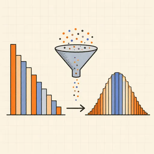
Central Limit Theorem Demo
Sample from any lopsided distribution and watch the averages pile up into a bell curve.
Conway’s Game of Life
Paint cells and watch Conway’s cellular automaton breed gliders, guns and oscillators.
Dynamic Geometry Board
Construct with points, lines, circles and transformations, then drag anything — the construction stays true, and a checker tells you which relations are theorems.

Fantasy Map Generator
Roll a seed and get a continent: coastlines, mountains, rivers, biomes and named towns, ready for your campaign.