The Double Pendulum, Explained
After reading this you will know exactly which equations the simulator integrates, why two nearly identical starts drift apart, and how to read the energy-drift number to judge whether the numbers on screen are still trustworthy.
What it is and why it misbehaves
A double pendulum is two rigid arms joined end to end, both free to swing in a vertical plane. The first arm hangs from a fixed pivot. The second arm hangs from the tip of the first. That is the whole machine: two rods, two masses, gravity. It looks like it should be as tame as a grandfather clock.
It is not. Release two copies from angles that differ by 10^{-4} radians (about 0.0057 degrees) and they trace the same curve for a few swings, then split and never agree again. That splitting is deterministic chaos. Nothing random happens. The equations are fixed, the integration is repeatable, yet long-term prediction fails because tiny differences grow exponentially.
The hook to try first: set the pendulum count to 60, give the arm a large release angle near the horizontal, and watch the single glowing tip fan out into a rainbow spray. Count the swings before the colors separate. That count is your first measurement of how fast this system forgets its starting condition.
When it is the right model, and when it is not
Use this simulator to build intuition about three things: sensitive dependence on initial conditions, the difference between a solvable and an unsolvable system, and how a numerical integrator conserves (or fails to conserve) energy over long runs.
Do not read it as a model of anything with friction, air drag, flexible arms, or joint slop. The equations here assume rigid massless rods, point masses, no damping, and a perfectly rigid pivot. A real pendulum loses energy every swing and eventually stops. This one never stops. If you want a system where damping is the point, the Harmonograph draws figures that decay on purpose.
Chaos is not the same as noise. Every run from the same numbers gives the same result on the same machine. What breaks is your ability to predict from an approximate start, because you never know the true angle to infinite precision.
The equations of motion
Let \theta_1 and \theta_2 be the angles of the two arms from vertical, m_1, m_2 the masses, L_1, L_2 the lengths, and g gravity. The angular accelerations come from the Euler-Lagrange equations. The first arm obeys:
Here \dot{\theta} is angular velocity and \ddot{\theta} is angular acceleration. The \sin(\theta_1-\theta_2) and \cos(2\theta_1-2\theta_2) terms are the coupling: the two arms push on each other, and that coupling is where the nonlinearity lives. The squared velocities \dot{\theta}_1^2 and \dot{\theta}_2^2 mean the equations are not just nonlinear in position but in speed too.
The second arm has a matching expression:
No combination of elementary functions solves these. That is not a gap in anyone's cleverness; it is a proven property of the system. The only way forward is to step time forward in small pieces, which is what the integrator does.
How the integrator steps time forward
The state is four numbers: \theta_1, \theta_2, \dot{\theta}_1, \dot{\theta}_2. Given the state now, the equations above tell you the four derivatives. Fourth-order Runge-Kutta (RK4) advances the state by a time step h using four slope estimates:
Here y is the four-number state, k_1 is the derivative at the start of the step, k_2 and k_3 are derivatives at the midpoint using progressively better guesses, and k_4 is the derivative at the end. The weighted average gives an error per step that shrinks like h^5. Halve the step and the local error drops by a factor of 32. This is why RK4 holds energy far better than a naive Euler step, though it still drifts a little over long runs.
Reproducing the demo defaults
The demo button uses the field defaults. Take m_1 = m_2 = 1, L_1 = L_2 = 1, g = 9.81, both arms released from rest at \theta_1 = \theta_2 = 90^\circ = \pi/2 radians.
- Total energy at release is potential energy only, since both velocities are zero. Measure height from the pivot. The first mass sits at height -L_1\cos\theta_1 = 0 (horizontal arm). The second sits at -L_1\cos\theta_1 - L_2\cos\theta_2 = 0 as well.
- So E = m_1 g y_1 + m_2 g y_2 = 0 joules using the pivot as zero. Any later reading should stay near
0. - Step the state with h = 0.005 seconds. After the first step the horizontal arm has started to fall, gaining a small negative height and matching negative potential offset by positive kinetic energy.
- Add the two rainbow copies at \theta_1 = \pi/2 + 10^{-4}. For the first second all copies overlap to the eye. Their angular separation grows roughly like 10^{-4} e^{\lambda t}, where the Lyapunov exponent \lambda for this setup is near
3per second. - Solve 10^{-4} e^{3t} \approx 1 for visible separation: t \approx \ln(10^4)/3 \approx 3.07 seconds. Expect the colors to split noticeably around three seconds in.
Reading the numbers on screen
Two readouts matter. The elapsed time tells you where you are on the divergence curve above. The energy and its drift tell you whether the integrator is still honest.
- Total energy
- The sum of kinetic and potential energy of the first pendulum. In the frictionless ideal this is a constant of motion for all time.
- Energy drift
- The difference between the current energy and the release energy. In exact math this is zero. In RK4 it wanders by a small amount that grows slowly with run length and shrinks fast when you reduce the step size.
- Lyapunov exponent
- The rate \lambda at which nearby trajectories separate, so separation scales like e^{\lambda t}. A positive value is the signature of chaos.
A practical rule: while the drift stays below about 0.1% of the release energy, trust the trajectory shape. Once drift climbs past a few percent, the on-screen swing is a plausible chaotic path but no longer the true path from your exact start.
Common mistakes
The first mistake is expecting two runs to match after the inner arm flips over the top. Once the first arm completes a full rotation, the accumulated exponential growth has amplified any difference (including rounding in the last bit of a floating-point number) to full scale. The paths are then unrelated.
The second mistake is blaming the integrator for the divergence between rainbow copies. That divergence is real physics, not numerical error. The integrator's own error shows up in the energy drift, not in the fan-out.
Do not run for minutes at a large step size and then read exact tip positions. The trajectory stays qualitatively correct, but a drift of several percent in energy means the specific path shown is no longer the path from your input. Shrink the step if you need a faithful long run.
The third mistake is treating a longer run as more informative. Past the point where drift and chaos have both grown, extra seconds add motion but no new predictive content.
Related simulations
If the coupling and resonance in this system interest you, several other simulators explore the same physics from other angles. The Wave Interference tank shows what happens when many simple oscillations add up. The Chladni Plate Patterns tool turns vibration modes into visible sand figures. For a many-body system where sensitivity to starting conditions also runs wild, try the Galaxy Collision Simulator. If you prefer a spring-and-mass network you can poke by hand, the Cloth Simulator integrates Verlet dynamics in real time.
Frequently asked questions
Why does the double pendulum have no formula for its position over time?
The equations of motion are nonlinear and coupled, mixing \sin(\theta_1-\theta_2) with squared angular velocities. No change of variables reduces them to something integrable in closed form. This is a proven result, not a missing trick, so numerical stepping is the only route.
Is the motion actually random?
No. It is fully deterministic. The same starting numbers always give the same path on the same machine. What is impossible is predicting far ahead from an approximate start, because errors grow like e^{\lambda t} with a positive \lambda.
What should the energy drift readout show?
Ideally zero, since the frictionless pendulum conserves energy exactly. In practice RK4 leaves a small drift. Keep it under about 0.1% of the release energy for a trustworthy trajectory, and halve the time step if it grows too large.
How many seconds until prediction becomes hopeless?
For the default setup with copies 0.0001 rad apart and \lambda \approx 3 per second, separation reaches about 1 radian near 3 seconds. After the inner arm's first flip, treat the specific path as unpredictable.
Does changing the masses or lengths change the chaos?
Yes. Chaos is strongest at large release angles where the arms can flip over the top. At small angles near vertical, the motion is nearly regular and the rainbow copies stay together far longer, because the effective Lyapunov exponent drops toward zero.
Related tools
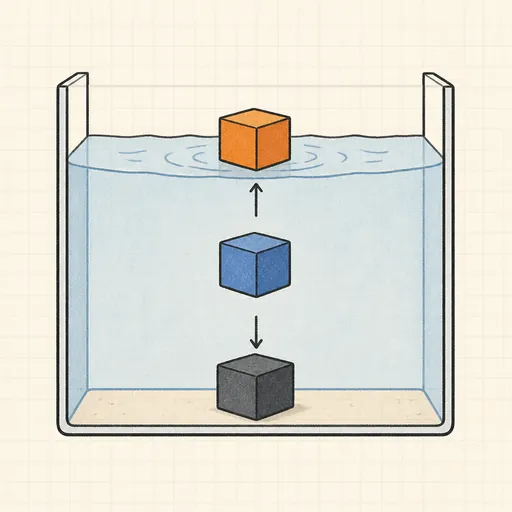
Buoyancy Tank
Drop blocks of different density into water and watch Archimedes decide what floats, sinks or hovers.
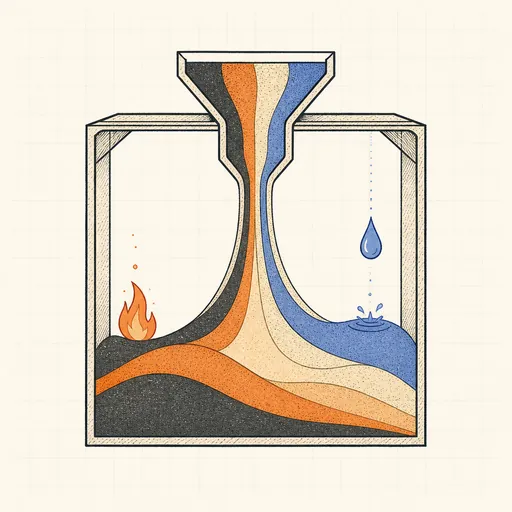
Falling-Sand Playground
Paint sand, water, oil, fire and more and watch them pour, settle, burn and react pixel by pixel.

Fluid Flow Simulator
Stir glowing dye through a real-time GPU fluid simulation.
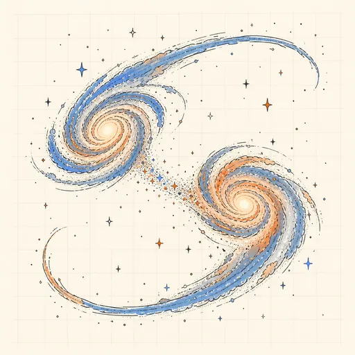
Galaxy Collision Simulator
Smash two spiral galaxies together and watch tidal tails and bridges form.
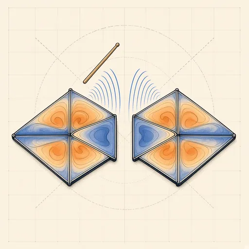
Hear the Shape of a Drum
Draw any drum and hear its true vibration modes — then meet two different drums that sound exactly the same.
Orbit Sandbox
Fling planets around a star and watch Newtonian gravity draw ellipses, slingshots and chaotic dances.