Ant Colony Pheromone Trails, Explained
After reading this you will understand how ants build foraging highways with no map and no leader, you will be able to derive the deposit-and-evaporation update rule on a grid, and you will know which parameter settings sharpen a trail versus dissolve it.
What the simulation shows
A colony of ants leaves the nest, wanders until someone finds food, and within a minute a bright line connects nest to food. No ant planned that line. Each ant follows two simple habits: drop a chemical marker as you walk, and steer toward the strongest marker ahead of you. The line is the visible sum of thousands of these small acts.
The trick that makes it work is that ants lay different markers depending on what they are doing. A searching ant drops a "to-home" scent, so it always knows the way back. A loaded ant carrying food drops a "to-food" scent, which is exactly the breadcrumb a searcher wants. Each field guides the other set of ants. The nest and the food act as fixed anchors, and the two scent fields grow toward each other in the middle.
This is stigmergy: coordination through traces left in a shared environment, rather than direct messages. The word was coined by Pierre-Paul Grassé in 1959 for termites, and the same idea drives this grid.
When this model is useful, and when it is not
Use this simulation to build intuition about positive feedback with a decay term. It is a clean laboratory for one question: when does reinforcement win against forgetting? That balance appears in real ant colonies, in routing algorithms (Ant Colony Optimization), and in any system where a signal is both amplified by use and erased by time.
Do not read it as biology at full resolution. Real ants use several pheromone species, trail geometry, polarized light, step counting, and antennal contact. This grid keeps two scalar fields and three sensors per ant. It reproduces the emergence of a trail and its collapse when food runs out. It does not predict a specific species' behavior, and it will not give you the true chemistry of the marker.
The double-bridge experiments of Deneubourg and Goss are the classic test. Give a colony two paths of different length to the same food and it converges on the shorter one, because ants on the short path complete the round trip faster and reinforce it more often per minute. This grid shows the same logic without an explicit graph.
The update rule and the intuition behind it
Two things happen to every scent field each time step: it fades everywhere, and it gains fresh deposits where ants walked. Write the pheromone value in grid cell (i,j) at time t as \tau_{ij}^{t}. The core rule is:
Here \rho is the evaporation rate per step, a number between 0 and 1. The factor (1-\rho) shrinks whatever was there. \Delta_{ij}^{t} is the total pheromone dropped into that cell during the step, which is the deposit amount q times the number of ants that visited. A blur pass usually follows, spreading a little scent to the eight neighbors so the gradient is smooth enough to sense.
An ant with no deposit reaching a cell leaves \tau decaying as a geometric sequence. Starting from \tau_0, after n empty steps the value is \tau_0 (1-\rho)^n. With \rho = 0.02 a trail keeps (0.98)^{100} \approx 0.133, about 13 percent, after 100 unused steps. It has a half-life you can compute directly:
For \rho = 0.02 that is \ln 0.5 / \ln 0.98 \approx 34.3 steps. A cell loses half its scent in about 34 steps if nobody refreshes it.
Steering uses three forward sensors placed at angles -\theta, 0, and +\theta from the ant's heading. The ant reads the target field at each sensor and turns toward the largest reading. If the center is largest it keeps going straight. Momentum plus a little random jitter keeps it from freezing in place and lets it explore.
A worked example with the demo defaults
The demo starts with default settings. Take the balance of deposit against evaporation for a single busy cell and follow it by hand. Assume the deposit is q = 1.0 per visiting ant, evaporation is \rho = 0.02 per step, and while food is plentiful an average of 3 ants cross this cell each step.
Does a well-used cell reach a stable trail strength?
Each step the cell gains 3 \times 1.0 = 3.0 and loses 2 percent of what it holds. The value climbs until gain equals loss.
- Start at
0. Step 1:0.98(0) + 3 = 3.000. - Step 2:
0.98(3) + 3 = 5.940. - Step 3:
0.98(5.940) + 3 = 8.821. - Step 10: the running formula gives
27.10. - Step 50:
140.5. - Equilibrium: set \tau^{*} = 0.98\,\tau^{*} + 3, so \tau^{*} = 3 / 0.02 = 150.
The cell saturates near 150. A cell with only 1 ant per step saturates at 1/0.02 = 50. That ratio, 150 to 50, is why a busy path looks three times brighter and pulls in still more ants. The general equilibrium is \tau^{*} = q\,v / \rho for v visits per step.
Explore the deposit-versus-evaporation balance
The single most instructive move is to change \rho and watch where the trail settles. Higher evaporation means a lower ceiling and a faster forget.
Reading the fields on screen
The teal field is the to-home scent, the amber field is the to-food scent, and amber-tinted ants are carrying food home. Watch the sequence in stages.
- Diffuse glow
- Early on, both fields are faint clouds around the nest. No ant has found food yet, so no to-food trail exists. Searching looks random.
- First thread
- The moment one ant reaches food and turns back, it lays a thin amber line. Nearby searchers lock onto it. This is the first positive feedback loop closing.
- Highway
- Traffic concentrates. The chosen path saturates near q v / \rho while side branches, visited by fewer ants, sit far lower and evaporate away. Contrast sharpens.
- Fade
- When the food pile shrinks to zero, deposits stop. The amber trail decays with half-life n_{1/2}, and ants disperse to search again.
A useful check: count how many steps the highway takes to fade after food is gone. With \rho = 0.02 and a saturated value of 150, it drops below a visible threshold of 10 after about \ln(10/150)/\ln 0.98 \approx 134 steps. Raise \rho to 0.1 and the same fade takes only \ln(10/30)/\ln 0.9 \approx 10.4 steps, because the ceiling is lower too.
Common mistakes when tuning
Setting evaporation to zero does not give you the strongest colony. It gives you a frozen map. Old trails never erase, so when food moves the ants keep marching to an empty spot. Every trail eventually reaches the maximum the field allows and the whole grid glows uniformly, which carries no gradient and no information.
The opposite error is evaporation set too high. If the half-life is shorter than a round trip from nest to food, a returning ant's fresh deposit has already faded before the next ant arrives, so the loop never closes. As a rule of thumb, keep n_{1/2} larger than the travel time in steps. If the trip is 60 steps, an \rho above roughly 0.011 (half-life 60) starts to hurt.
Two more traps. A sensor angle \theta that is too narrow makes ants nearly blind to a trail just off their heading, so they miss it; too wide and they oversteer and weave. A deposit amount so large that cells saturate in one or two visits erases the difference between busy and quiet paths, since both hit the ceiling, and the colony cannot choose. Keep deposits small enough that many visits are needed to saturate.
Related simulations on this site
The same self-organizing spirit runs through several other models here. Slime Mould Networks uses agents that deposit and follow a single trail field, the closest cousin to this colony. Boids Flocking Simulator gets group motion from three local rules with no shared field at all. Firefly Synchronization shows coupling through pulses instead of chemistry. For growth-based networks try Mycelium Growth, and for pure emergent pattern in a continuous grid see Lenia Continuous Life. If you want selection rather than signaling, Evolving Creatures and the Genetic Drift Simulator shift the focus to populations over generations, and Neuron Action Potential and L-System Plants round out the biology set.
Frequently asked questions
Why do the ants use two separate pheromones?
One field alone cannot tell an ant which way is home versus which way is food. Searching ants lay to-home scent and follow to-food scent; loaded ants do the reverse. Each group builds the trail the other group needs, and the two fields meet in the middle to form a two-way road.
What happens if I set evaporation to zero?
Trails stop erasing. The colony cannot forget an exhausted food source, and over time the whole field saturates near its maximum, wiping out the gradient the ants read. You get a bright frozen grid with no useful structure.
How fast does a trail disappear after food runs out?
It decays geometrically as \tau_0 (1-\rho)^n. The half-life is \ln 0.5 / \ln(1-\rho): about 34 steps at \rho = 0.02, about 7 steps at \rho = 0.1.
Does more ants always mean a stronger trail?
Up to a point. Equilibrium strength is q v / \rho, so more visits v raise the ceiling linearly. Past saturation, though, every path hits the maximum and the colony loses its ability to prefer the shorter route.
Is this how real ants navigate?
Partly. Real ants do lay and follow pheromones, and the shortest-path result is well documented. But they also use vision, step counting, and direct contact, and they use several chemical signals. Treat this grid as a clean model of one mechanism, not a full account of ant behavior.
Related tools
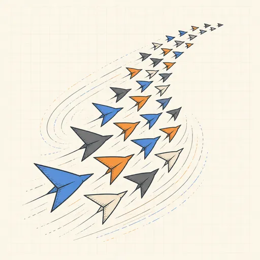
Boids Flocking Simulator
Watch lifelike flocking emerge from three local rules with Reynolds’ boids model.
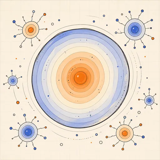
Lenia Continuous Life
Grow smooth self-organising lifeforms like the gliding Orbium in a continuous cellular automaton.
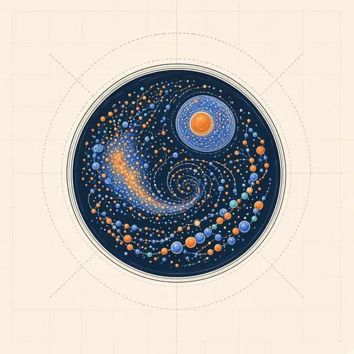
Particle Life
A few coloured species and one table of likes and dislikes — and cells, chains and chasing creatures emerge by themselves.
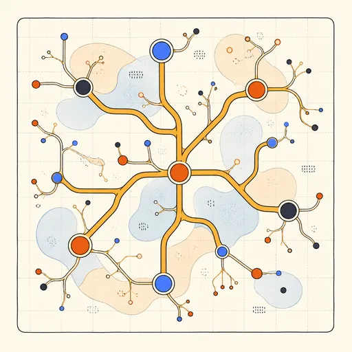
Slime Mould Networks
Watch millions of Physarum agents self-organise into living transport networks.
Evolving Creatures
See natural selection reshape a population of foraging creatures generation by generation.
Firefly Synchronization
See a meadow of fireflies fall into spontaneous unison as pulse-coupled oscillators.