Hierarchical Clustering and the Dendrogram, Explained
After reading this you can build a merge tree from a handful of points by hand, read where the tree wants you to cut it, and tell when single linkage will chain two real clusters into one.
What hierarchical clustering does
Agglomerative hierarchical clustering starts with every point as its own cluster. It then repeats one step: find the two closest clusters and merge them. With n points that step runs n - 1 times, until a single cluster holds everything. The record of which clusters merged, and at what distance, is a binary tree called a dendrogram.
The tree is the whole answer. You do not pick the number of clusters before running the algorithm. You run it once, then cut the tree at whatever height you like. A high cut leaves a few large clusters; a low cut leaves many small ones. One tree answers every choice of cluster count.
Here is the hook. Take the two moons preset: two interleaved crescents. Run single linkage and each crescent stays whole, because single linkage merges along the nearest edge and follows the curve. Run Ward on the same points and the crescents get sliced into round blobs, because Ward wants compact clusters. Same data, same algorithm skeleton, different linkage, opposite result.
When to use it, and when not
Reach for hierarchical clustering when you want the whole nesting structure, not just a flat partition. It answers "which groups merge first, and at what distance" in one picture. It needs no guess at the cluster count up front, and it accepts any distance matrix, so you can cluster things that are not points in space (edit distance between strings, correlation between stocks) as long as you can define a pairwise distance.
Avoid it at scale. The naive method used in the tool is O(n^3) time and O(n^2) memory: fine for 60 points, hopeless for a million. It is also greedy. Once two clusters merge, they never split, so an early mistake propagates up the tree.
If you have tens of thousands of points and roughly round clusters, use k-Means Clustering instead, which scales far better. If your clusters are irregular blobs separated by empty space, try DBSCAN Clustering, which also labels outliers as noise.
Linkage: four ways to measure cluster distance
Merging needs a distance between clusters, not just between points. Given clusters A and B and the pairwise point distances between them, the four choices are:
- Single
- The minimum pairwise distance: \min_{a \in A, b \in B} d(a,b). Merges along the nearest pair.
- Complete
- The maximum pairwise distance: \max_{a \in A, b \in B} d(a,b). Merges by worst case, so it keeps clusters tight.
- Average
- The mean over all cross pairs: \frac{1}{|A||B|} \sum_{a,b} d(a,b). A compromise between single and complete.
- Ward
- Merge the pair that increases total within-cluster variance by the least. It favors compact, roughly equal-sized clusters.
All four update the distance matrix after a merge with a single recurrence, the Lance-Williams formula. When clusters i and j merge, the distance from the new cluster to any other cluster k is:
Here d(i,k) and d(j,k) are the old distances, d(i,j) is the distance at which i and j just merged, and the four coefficients pick the linkage. Single uses \alpha_i = \alpha_j = \tfrac{1}{2}, \beta = 0, \gamma = -\tfrac{1}{2}, which turns the bracket into a minimum. Complete flips \gamma to +\tfrac{1}{2} to get a maximum. Average sets \alpha_i = |i|/(|i|+|j|) weighted by cluster size, with \beta = \gamma = 0. Ward uses size-dependent coefficients that track variance.
A worked example on three points
Building a tiny dendrogram by hand
Take three points on a line so the arithmetic stays checkable: P_1 = 0, P_2 = 1, P_3 = 4. Distances are absolute differences.
- Start with three clusters. Pairwise distances: d(1,2) = 1, d(1,3) = 4, d(2,3) = 3.
- The smallest is d(1,2) = 1. Merge P_1 and P_2 at height
1. That is the first junction. - Now update the distance from the new cluster \{1,2\} to P_3. With single linkage it is \min(4, 3) = 3. With complete linkage it is \max(4, 3) = 4. With average linkage it is (4 + 3)/2 = 3.5.
- Only two clusters remain, so merge them. The top junction sits at height
3for single,4for complete,3.5for average.
The tree shape is identical for all three linkages here (first \{1,2\}, then join P_3). Only the top junction's height differs. That gap, 3 versus 4 versus 3.5, is exactly the disagreement each linkage introduces about how far apart the two final clusters are.
Cutting the tree and reading the result
To turn a tree into a flat clustering, draw a horizontal line at some height and count the vertical branches it crosses. Each crossed branch below the line is one cluster. In the three-point example, a cut at height 2 crosses two branches (the \{1,2\} branch and the lone P_3 branch), giving two clusters. A cut at height 0.5 crosses all three branches, giving three singleton clusters. A cut above the top junction gives one cluster.
The vertical height of a junction is the distance at which that merge happened. Tall vertical segments mean a merge that joined two clusters that were far apart, which is a hint of real separation. The trick for choosing a cut count: look for the tallest vertical gap that no junction interrupts, and cut through it. Cutting through a large gap is stable, because sliding the line up or down within the gap does not change the cluster count.
The dendrogram does not fix a left-to-right order of leaves. Software can flip any junction's two children without changing the tree, so two correct dendrograms of the same data may look mirrored. Read heights and groupings, never horizontal position.
The chaining trap of single linkage
Single linkage looks only at the nearest pair of points between two clusters. That makes it follow thin, curved shapes, which is why it keeps each moon whole. The same property is its weakness. A single stray point sitting halfway between two well-separated clusters creates a short hop from cluster A to the stray, and another short hop from the stray to cluster B. Single linkage takes both hops and fuses A and B into one cluster, even though the bulk of A is far from the bulk of B. This is chaining.
Concretely, suppose cluster A is a tight ball near x = 0 and cluster B is a tight ball near x = 10, and you drop one bridge point at x = 5. Single linkage sees a maximum hop of about 5 along the chain A \to 5 \to B and merges everything early. Complete linkage measures A-to-B by their farthest pair, about 10, so it resists the merge and keeps the balls apart. Ward, driven by variance, also keeps them apart. If your data has bridging noise, prefer complete or Ward, or clean the noise first.
Common mistakes
Three errors account for most bad hierarchical clusterings.
- Unscaled features. Distance mixes all dimensions. If one feature spans 0 to 1000 and another spans 0 to 1, the big one dominates every distance and the small one is invisible. Standardize features to comparable scales before clustering.
- Ward with a non-Euclidean distance. Ward is defined through variance, which assumes squared Euclidean distance. Feeding it correlation or cosine distances produces heights that do not mean what you think. Use average or complete linkage for those.
- Cutting at a fixed count out of habit. Forcing three clusters when the tallest gap in the tree clearly splits the data into two means you are cutting through a short gap, where the count is unstable and a tiny data change flips points between clusters.
Do not read a low junction as strong evidence of a cluster. Low junctions merge points that were already close, which is expected. Evidence of real structure is a tall junction sitting above a wide empty gap. Judge merges by the height of the jump, not by how early they happen.
Related tools
Hierarchical clustering is one of several ways to group unlabelled points, and comparing them on the same data teaches more than any single method alone.
Gaussian Mixture & EM fits soft, elliptical clusters and gives each point a membership probability instead of a hard label. Self-Organizing Map lays a neuron grid over the data to preserve neighbourhood structure. For seeing high-dimensional clusters before you cluster them, t-SNE Explorer and PCA Toy both project down to 2D, one by preserving local neighbours and one by preserving variance. If your real question is which points are outliers rather than which group they belong to, the Anomaly Detection Playground scores that directly.
Frequently asked questions
How do I choose the number of clusters from a dendrogram?
Find the tallest vertical stretch that no junction crosses, and put the cut inside it. Count the branches the cut crosses; that is your cluster count. In the three-point example, the gap between height 1 and height 3 is the tallest clear span, so cutting there gives two clusters and is stable across that whole range.
Which linkage should I use by default?
Ward is a reasonable first try when your clusters are roughly round and you use Euclidean distance, because it produces compact, balanced clusters. Use single linkage only when you actually expect long, thin, or curved shapes, and only if your data has little bridging noise. Complete and average sit between the two.
Why does single linkage keep the moons together but Ward splits them?
Single linkage merges by the nearest pair of points, so it walks along the edge of each crescent and never jumps the gap to the other moon. Ward merges to minimize variance, and a crescent has high variance, so Ward prefers to slice it into two compact halves instead of keeping the curved shape.
Can hierarchical clustering handle a million points?
Not with the naive method, which needs O(n^2) memory for the distance matrix and O(n^3) time. A million points would need on the order of a trillion distance entries. Use k-means or a sampling scheme at that scale, and reserve hierarchical clustering for up to a few thousand points.
Does the algorithm ever undo a merge?
No. Agglomerative clustering is greedy: once two clusters merge they stay merged for the rest of the run. That is why an early merge caused by a noise point can distort the whole upper tree, and why cleaning outliers before clustering matters.
Related tools
Distribution Sketcher
Sketch the shape of a probability density — or paste raw data — and search 16 distributions for the ones that fit it best.
PCA Toy
Find the axes of maximum variance and flatten a point cloud onto them.
k-Means Clustering
Step through Lloyd’s algorithm and watch centroids chase the middles of your point clouds.
Anomaly Detection Playground
Flag outliers three different ways and see where each score breaks down.
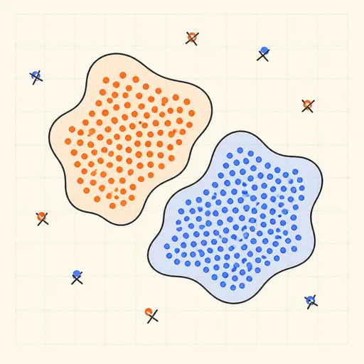
DBSCAN Clustering
Grow density-based clusters point by point and watch noise get left behind.
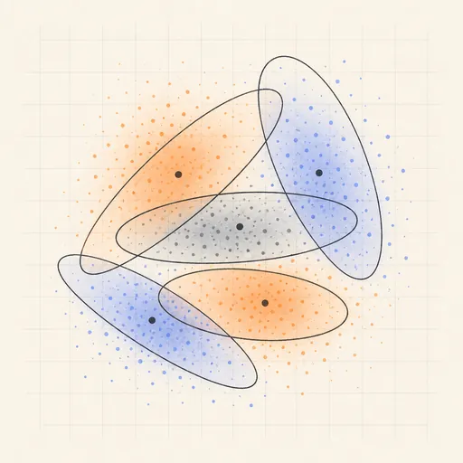
Gaussian Mixture & EM
Fit soft, elliptical clusters with the expectation–maximization algorithm.