Gaussian Mixtures and the EM Algorithm, Explained
After reading this you can explain what a Gaussian mixture model assumes about your data, run the two EM steps by hand on a tiny dataset, read the responsibilities and covariance ellipses, and know when a mixture beats plain k-means and when it fails.
What a Gaussian mixture model is
A Gaussian mixture model (GMM) treats your data as if it came from k overlapping Gaussian bells. Each bell has three things: a weight (how much of the data it accounts for), a mean (its center), and a covariance (its size, shape and tilt). A point is not assigned to one cluster outright. Instead it gets a set of membership probabilities, one per component, that sum to 1. That soft assignment is the main difference from k-means, which forces each point into exactly one cluster.
Here is the hook. Take two clusters shaped like long tilted cigars that cross near the middle. k-means draws a straight boundary halfway between the two centers and slices both cigars in the wrong place, because it only knows round, equal-size blobs. A GMM with full covariance learns the tilt and the elongation, so its ellipses hug each cigar along its own axis. Same data, very different fit, because the model of a cluster is richer.
When to use it, and when not
Reach for a GMM when clusters overlap, when they have different sizes or shapes, or when you want a probability rather than a hard label. Density estimation is another use: once fit, the model gives you p(x) everywhere, which you can threshold to flag low-density points as anomalies.
Avoid a GMM when your clusters are not even roughly elliptical. Two concentric rings or a pair of interlocking crescents break the Gaussian assumption, and no covariance matrix will fix that. Density-based methods handle those shapes far better. A GMM also needs you to pick k in advance, and it can be slow and unstable with many components in high dimensions, where each full covariance costs d(d+1)/2 parameters.
A Gaussian mixture assumes each cluster is a single elliptical bell. If your data has non-convex or nested shapes, the fit will look confidently wrong. Plot the ellipses before you trust the labels.
The two steps and their formulas
EM alternates between guessing memberships and refitting parameters. Start with the membership probabilities, called responsibilities. For point x_i and component k:
Here \pi_k is the weight of component k, \mu_k its mean, \Sigma_k its covariance, and \mathcal{N} the Gaussian density. The numerator is the joint probability that the point belongs to component k; dividing by the sum over all components normalizes the responsibilities so they add to 1. This is the E-step (expectation).
The M-step (maximization) refits each component using the data weighted by those responsibilities. Let N_k = \sum_i r_{ik} be the effective count of points in component k. Then:
The weight \pi_k is the fraction of the effective count. The mean is a responsibility-weighted average of the points. The covariance is a responsibility-weighted spread around that mean. Points that half-belong to a component contribute half their weight to it. That single idea, weighting by r_{ik} instead of a hard 0 or 1, is the whole trick.
A worked example you can reproduce
Use the tool's Well-separated preset feel with tiny numbers so you can check every arithmetic step by hand. Take five points on a line and fit k = 2 with spherical covariance.
One EM iteration on five points
Data: x = [0, 1, 2, 8, 9]. Initialize means at \mu_1 = 1 and \mu_2 = 8, equal weights 0.5, and variance \sigma^2 = 4 for both, so \sigma = 2.
- E-step for
x = 2. The squared distances are (2-1)^2 = 1 and (2-8)^2 = 36. The unnormalized densities use \exp(-d/(2\sigma^2)) = \exp(-d/8): component 1 gives e^{-0.125} = 0.8825, component 2 gives e^{-4.5} = 0.0111. - Normalize: r_{1} = 0.8825/(0.8825+0.0111) = 0.9876, so r_{2} = 0.0124. Point
2is almost entirely in cluster 1. - By the same arithmetic, points
0and1get responsibility above0.999for cluster 1, and points8and9above0.999for cluster 2. The clusters are so far apart that the soft assignment is nearly hard. - M-step means. Treat the near-
1responsibilities as1. New \mu_1 = (0+1+2)/3 = 1.0 and new \mu_2 = (8+9)/2 = 8.5. - M-step weights. Effective counts are about
3and2, so \pi_1 \approx 0.6 and \pi_2 \approx 0.4.
Run a second iteration and the means barely move, because the responsibilities were already almost binary. That is convergence on easy data: EM reaches it in one or two passes.
Now imagine sliding the two groups toward each other. The point at 2 would earn a responsibility like 0.7 instead of 0.99, and its 0.3 share would pull the second mean leftward. That partial pull is exactly what k-means cannot do.
Watching the log-likelihood climb
EM does not minimize a distance. It maximizes the log-likelihood of the data under the mixture:
Each term is the log of the total density the mixture assigns to one point. A well-placed model gives every point high density, so the sum is large (less negative). The key guarantee: every full EM iteration increases \log L or leaves it unchanged, never decreases it. That is why the mini-chart rises monotonically and then flattens.
Monotone does not mean optimal. EM climbs to a local maximum that depends on where you started, exactly like k-means. Run it several times from different initial means and keep the fit with the highest final log-likelihood.
Reading the ellipses and responsibilities
Two things carry the meaning of a fit: the ellipses and the colors.
- 1σ and 2σ ellipses
- Each ellipse is a contour of constant density. The
1σellipse encloses roughly39%of a 2D Gaussian's mass, the2σellipse roughly86%. Their orientation comes from the eigenvectors of \Sigma_k; their axis lengths come from the square roots of the eigenvalues. - Responsibility (soft membership)
- A point colored a clean single hue has responsibility near
1for that component. A point blended between two hues sits in the overlap, with responsibilities like0.55and0.45. These blends live near the crossing of two ellipses. - Covariance type
- Spherical forces round clusters (one variance, equal in every direction). Full allows tilt and elongation (a general 2 \times 2 matrix). On the elongated preset only full covariance can hug the tilted clusters.
Common mistakes
Four pitfalls account for most bad GMM fits.
- Collapsing components. If one component latches onto a single point, its covariance shrinks toward zero, the density at that point shoots up, and the log-likelihood runs to +\infty. This is a degenerate solution, not a good one. The demo adds a small constant to each covariance diagonal to block it; in libraries this is the
reg_covarparameter. - Wrong covariance type. Fitting spherical components to elongated data forces round ellipses that cannot tilt, so the model splits one long cluster into several round pieces. Use full covariance for tilted or stretched clusters.
- Reading responsibilities as certainty. A responsibility of
0.9is a model estimate, not a fact. If the components overlap heavily, even confident-looking numbers can flip when you reinitialize. - Fixing k badly. Too few components merge distinct groups; too many carve one group into slivers. Compare fits across
kusing a penalized score such as BIC rather than the raw log-likelihood, which always improves as you add components.
Related tools
A GMM sits in a family of clustering and projection methods. Compare it with these to see the tradeoffs.
- k-Means Clustering is the hard-assignment limit of a GMM with spherical, vanishing covariance. Watching Lloyd's algorithm side by side shows exactly what soft membership adds.
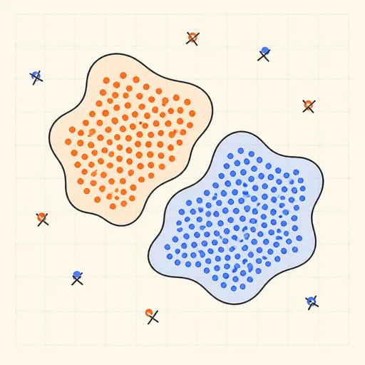
- DBSCAN Clustering finds clusters by density, so it handles the rings and crescents a GMM cannot.
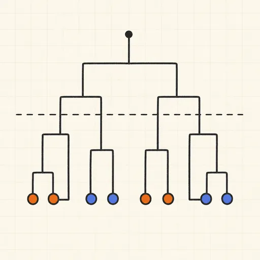
- Hierarchical Clustering & Dendrogram builds a merge tree and lets you cut it at any level, with no need to fix
kup front. - PCA Toy finds the axes of maximum variance, the same eigenvectors that orient a full covariance ellipse.
- t-SNE Explorer untangles high-dimensional clusters into 2D so you can eyeball how many components you might need.
- Self-Organizing Map maps data onto a neuron grid, a different route to seeing cluster structure.
- Anomaly Detection Playground uses low density (which a fitted GMM provides) as one of several outlier scores.
Frequently asked questions
How is a Gaussian mixture different from k-means?
k-means gives each point one label based on the nearest center and assumes round, equal-size clusters. A GMM gives each point a probability of belonging to every component and can fit tilted, elongated ellipses of different sizes. k-means is the special case of a GMM with spherical covariance shrunk to zero, where responsibilities harden to 0 or 1.
Why does the log-likelihood never go down?
EM is built so that each iteration maximizes a lower bound on the log-likelihood that touches the true value at the current parameters. Improving that bound cannot decrease the true log-likelihood. So the curve is monotone by construction, though it only reaches a local maximum.
How do I choose k?
Do not use the raw log-likelihood, which always rises as you add components. Fit several values of k and compare a penalized score like BIC, which subtracts a term for the number of parameters. Pick the k with the best score, and sanity-check the ellipses visually.
What does a responsibility of 0.6 actually mean?
It is the model's estimated probability that the point was generated by that component, given the current parameters. A point with responsibilities 0.6 and 0.4 sits in the overlap between two clusters. It is a statement about the model, not a measured truth.
Why does the demo add a small number to the covariance?
Without it, a component can collapse onto one point, driving its covariance to zero and the likelihood to infinity, a useless degenerate fit. Adding a small constant to the diagonal keeps every covariance invertible and the optimization stable.
Related tools
Distribution Sketcher
Sketch the shape of a probability density — or paste raw data — and search 16 distributions for the ones that fit it best.
PCA Toy
Find the axes of maximum variance and flatten a point cloud onto them.
k-Means Clustering
Step through Lloyd’s algorithm and watch centroids chase the middles of your point clouds.
Anomaly Detection Playground
Flag outliers three different ways and see where each score breaks down.
DBSCAN Clustering
Grow density-based clusters point by point and watch noise get left behind.
Hierarchical Clustering & Dendrogram
Merge points bottom-up and cut the dendrogram wherever you like.