3D Surface Plotter, Explained
After reading this, you will be able to read a function of two variables as a surface, spot its peaks, pits and saddle points by eye, and know why the ripple \sin(r)/r makes rings that fade with distance.
What a surface plot shows
A function of one variable, like y = x^2, draws a curve in the plane. A function of two variables, like z = x^2 - y^2, assigns a height z to every point (x, y) on the floor. Plot that height as elevation and you get a surface. The plotter builds this surface as a mesh of small quadrilaterals and colours each point by height, so you can rotate it and look underneath.
Start with the saddle z = x^2 - y^2. Walk east along the x-axis (set y = 0) and the height is z = x^2, a valley that curves upward. Walk north along the y-axis (set x = 0) and the height is z = -y^2, a ridge that curves downward. At the origin the surface goes up one way and down the other. That crossing shape is the saddle, and it is the single most useful thing this tool trains your eye to recognise.
When a surface plot helps, and when it misleads
Reach for a surface plot when you have a smooth function of exactly two inputs and you care about its shape: where it is high, where it is flat, how steep the slopes are, whether there are hidden saddles. It is the fastest way to check the geometry of a formula before you trust any calculation about it.
It stops helping in three cases. First, functions of three or more variables cannot be drawn this way, because you run out of spatial axes. Second, functions with sharp jumps or true singularities render as spikes that the finite mesh cannot resolve honestly. Third, a coarse grid can hide fast wiggles: if you sample \sin(20x) on a grid spaced 1 apart, you miss every oscillation and see nonsense. Match the grid to the smallest feature you expect.
A smooth-looking surface is not proof of smooth behavior. The mesh connects sample points with flat panels, so it can bridge right over a narrow spike or a discontinuity. If a formula has a denominator that hits zero, check what happens near that point by hand before you believe the picture.
The formula and the intuition behind height
Every surface here is a graph of the form below.
Here x and y are the two floor coordinates and z is the height plotted upward. The colour at each point encodes z directly, so warm and cool bands are level sets: all the points at one height share a colour, exactly like contour lines on a map.
The features you hunt for live where the surface goes flat in every direction. Those are the critical points, where both partial derivatives vanish.
The symbol \partial f / \partial x is the slope of the surface if you walk in the x-direction only, holding y fixed. A critical point can be a local maximum (a peak), a local minimum (a pit), or a saddle. To tell them apart you look at the curvature, captured by the second derivatives in what is called the Hessian.
Here f_{xx} is the x-direction curvature, f_{yy} the y-direction curvature, and f_{xy} the twist. If D \gt 0 and f_{xx} \gt 0 you have a pit; if D \gt 0 and f_{xx} \lt 0 you have a peak; if D \lt 0 you have a saddle, because the two directions curve opposite ways.
Working the saddle by hand
Classifying the origin of z = x² − y²
The demo defaults render this saddle. Reproduce its classification with four short steps.
- First derivatives: f_x = 2x and f_y = -2y. Both are zero only at
(0, 0), so the origin is the sole critical point. - Second derivatives: f_{xx} = 2, f_{yy} = -2, f_{xy} = 0.
- Discriminant: D = (2)(-2) - 0^2 = -4. Since D \lt 0, the origin is a saddle.
- Check with sample heights. At
(1, 0), z = 1. At(0, 1), z = -1. At(0, 0), z = 0. The origin sits above its north-south neighbours and below its east-west neighbours, so it is neither a peak nor a pit.
Reading the ripple and the peak
The ripple z = \sin(r)/r, where r = \sqrt{x^2 + y^2} is distance from the center, is the surface version of the sinc function. At the center the formula is 0/0, but the limit is well defined: as r \to 0, \sin(r)/r \to 1. So the surface peaks at height 1 in the middle. The rings sit where \sin(r) = 0, that is at r = \pi \approx 3.142, r = 2\pi \approx 6.283, and so on. Between rings the amplitude falls off like 1/r, so the first trough near r \approx 4.49 reaches about \sin(4.49)/4.49 \approx -0.217, and the ripples shrink from there.
The Gaussian peak z = e^{-(x^2 + y^2)} is a single smooth hill. Its height is 1 at the center and falls to e^{-1} \approx 0.368 at radius 1, and to e^{-4} \approx 0.0183 at radius 2. It never reaches zero but gets small fast. It has one critical point, a maximum, and no saddles.
| radius r | saddle on x-axis | ripple sin(r)/r | Gaussian e^(-r²) |
|---|---|---|---|
| 0 | 0 | 1 | 1 |
| 1 | 1 | 0.8415 | 0.3679 |
| 2 | 4 | 0.4546 | 0.01832 |
| 3.142 | 9.870 | 0 | 0.00005166 |
| 4.49 | 20.16 | -0.2172 | 0.0000000018 |
Reading colour, steepness and critical points
Colour bands are your contour map. Where the bands are packed tightly, the surface is steep, because a small step across the floor changes the height a lot. Where bands are wide and sparse, the surface is nearly flat. On the Gaussian, the bands crowd at radius 0.7 where the slope is steepest, and spread out both at the flat summit and out in the tail.
To find a saddle by eye, rotate until you see a point where the surface curves toward you along one line and away from you along the perpendicular line. The colour there sits between the warm high ground and the cool low ground, a pinch point in the middle of the palette. The monkey saddle z = x^3 - 3xy^2 is a trickier case: it has three valleys and three ridges meeting at the origin, so a monkey has somewhere to rest its two legs and its tail. Its discriminant test fails because all second derivatives vanish at the origin, which is why you need to look at the shape directly rather than trusting the quick D rule.
Spin the surface so your line of sight grazes along it, nearly edge-on. Flat regions and gentle saddles that are invisible from straight above pop into relief when you view them from a low angle.
Common mistakes
Confusing a saddle with a peak or pit is the classic error. From directly above, both look like a coloured bump. Only rotation reveals the opposite curvatures. Always check two perpendicular slices before you name a critical point.
The second mistake is trusting a coarse grid. The crossing waves surface z = \sin(x)\sin(y) has features spaced about \pi \approx 3.14 apart. Sample it on a grid coarser than about 0.5 and the peaks shift or vanish. If a surface looks jagged where you expect smoothness, refine the grid before drawing conclusions.
The third is reading the vertical scale as absolute. Plotters usually rescale z to fit the box, so a Gaussian topping out at 1 and a saddle reaching 25 can look the same height on screen. Check the axis numbers, not the visual height, when you compare surfaces.
Related tools
If you want the two-variable idea turned into flow rather than height, the Vector Field Visualizer shows the gradient as arrows, and the Slope Field Explorer does the one-variable analogue for differential equations. For surfaces that evolve in time, the Heat Equation Simulator watches a bump flatten out. To spin other 3D objects and build the same rotational intuition, try the Lorenz Attractor, the Tesseract Projection and the Platonic Solids Explorer. If the colour-as-height idea appeals, the Mandelbrot Explorer colours the plane by a very different rule.
Frequently asked questions
Why does sin(r)/r not blow up at the center?
Because near zero, \sin(r) \approx r - r^3/6, so \sin(r)/r \approx 1 - r^2/6, which heads to 1 as r goes to 0. The apparent 0/0 has a finite limit, and the surface has a smooth peak of height 1 at the center.
What is the difference between a saddle and a monkey saddle?
An ordinary saddle x^2 - y^2 has two directions up and two directions down, alternating around the point. The monkey saddle x^3 - 3xy^2 has three up and three down, so the pattern repeats every 120 degrees instead of every 90.
How do I know if a critical point is a peak, pit or saddle?
Compute the discriminant D = f_{xx} f_{yy} - (f_{xy})^2. Positive D with upward curvature is a pit, positive D with downward curvature is a peak, negative D is a saddle. If D = 0 the test is inconclusive and you must inspect the shape, as with the monkey saddle.
Why do the colour bands mean steepness?
Each band spans a fixed range of height. Where the surface climbs fast, you cross many bands over a short horizontal distance, so they look crowded. Where it is flat, one band covers a wide area. This is exactly how contour lines work on a topographic map.
Can this plot functions of three variables?
No. A graph needs one axis per input plus one for the output, so two inputs already use all three spatial axes. For three inputs you would need a fourth dimension, which is why higher-variable functions are studied through slices, level sets or projections instead.
Related tools
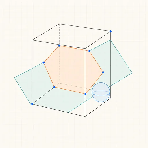
3D Geometry Board
Points, lines, planes, spheres and polyhedra on an orbiting camera — slice solids with planes, unfold nets, drop the Dandelin spheres into a cone and drag everything.
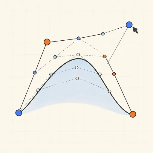
Bézier Curve Playground
Drag control points and watch De Casteljau’s algorithm construct a Bézier curve step by step.
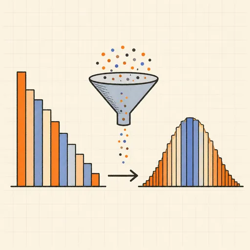
Central Limit Theorem Demo
Sample from any lopsided distribution and watch the averages pile up into a bell curve.
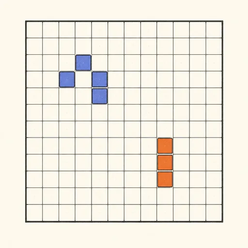
Conway’s Game of Life
Paint cells and watch Conway’s cellular automaton breed gliders, guns and oscillators.
Dynamic Geometry Board
Construct with points, lines, circles and transformations, then drag anything — the construction stays true, and a checker tells you which relations are theorems.
Fantasy Map Generator
Roll a seed and get a continent: coastlines, mountains, rivers, biomes and named towns, ready for your campaign.