Small-World Networks, Explained
After reading this you will know how one rewiring probability turns a village-like ring lattice into a network you can cross in a handful of hops, how to compute the path length and clustering that define the small-world regime, and how to read the two curves the lab plots.
What a small world is, and one hook example
Pick two strangers anywhere on Earth. In 1967 Stanley Milgram asked people in Nebraska to forward a letter toward a target in Boston, passing it only to someone they knew on a first-name basis. The chains that arrived took a median of about six steps. That is the origin of "six degrees of separation."
The puzzle is that your social world does not look like it should allow this. Your friends mostly know each other. That is high clustering: dense local triangles, like a village. A pure village should be slow to cross, because you can only step to a neighbour of a neighbour. Yet the whole planet is reachable in six hops.
In 1998 Duncan Watts and Steven Strogatz resolved the tension with one construction and one knob. Start from a ring of N nodes where each node connects to its k nearest neighbours. Then walk over every edge and, with probability p, rewire one end to a random node. A tiny p plants a few long-range shortcuts. Those shortcuts barely touch the local triangles, but they slash the number of hops needed to cross the network. The Small-World Network Lab draws this live and sweeps p so you can watch both effects at once.
When the model applies, and when it does not
Use the Watts-Strogatz model when you want the cleanest possible demonstration of one fact: that a small fraction of long-range links produces short paths without destroying local structure. It is a teaching model. It explains why real graphs can be both clustered and short.
Do not use it as a fitted model of a specific real network. Real graphs have degree hubs: a few nodes with thousands of links. Watts-Strogatz gives every node nearly the same degree (each keeps close to k connections), so it cannot reproduce the heavy-tailed degree distribution of the web or of citation graphs. For that you want a preferential-attachment (Barabasi-Albert) model. The small-world lab answers a different question: given local structure, how few shortcuts buy you a short world?
Two graphs can share the same number of nodes and edges yet feel completely different. The ring lattice and the random graph in this lab both have Nk/2 edges. What changes as you slide p is only where those edges point, and that alone moves the average path length by a factor of dozens.
The two numbers that define a small world
Everything rests on two graph statistics.
- Average path length L
- The mean number of hops on the shortest path between two nodes, averaged over all pairs. Small L means the network is easy to cross.
- Clustering coefficient C
- For each node, the fraction of its neighbour pairs that are themselves connected. Averaged over all nodes. High C means dense local triangles.
For the starting ring lattice at p = 0, both have closed forms. The path length grows linearly with size:
Here N is the node count and k the number of neighbours each node connects to. To reach the far side of the ring you step k/2 nodes per hop, so crossing half the ring takes about N/2k hops.
The clustering of the ring is nearly constant, close to 3/4 for large k:
At the other extreme, p = 1, the graph is essentially random. Now path length grows only with the logarithm of size, and clustering collapses toward a tiny value:
The gap between logarithmic and linear growth is the whole story. For N = 1000 and k = 10, L(0) \approx 50 while L(1) \approx 3. The lab plots the normalised curves L(p)/L(0) and C(p)/C(0) so both start at 1.0 and fall as p rises. The signature is that the L curve drops almost at once while the C curve holds flat far longer.
A worked example reproducing the demo
From village to small world with N = 1000, k = 10
The demo button uses the field defaults: N = 1000 nodes, k = 10 neighbours each. Work the anchor values by hand.
- Path length at p = 0: L(0) \approx N/2k = 1000/20 = 50 hops.
- Clustering at p = 0: C(0) = 3(k-2)/(4(k-1)) = 3 \cdot 8 / (4 \cdot 9) = 24/36 = 0.6667.
- Path length at p = 1: L(1) \approx \ln 1000 / \ln 10 = 6.908 / 2.303 = 3.0 hops.
- Clustering at p = 1: C(1) \approx k/N = 10/1000 = 0.01.
Now the intermediate regime. Barrat and Weigt give an approximation for clustering under rewiring: C(p) \approx C(0)(1-p)^3, since a triangle survives only if all three of its edges avoid rewiring. Path length has no simple closed form, but it drops steeply. At p = 0.01 the network already carries roughly pNk/2 = 0.01 \cdot 5000 = 50 shortcut edges, enough to cut L to about 8 or 9 hops. Meanwhile C(0.01) \approx 0.6667 \cdot 0.99^3 = 0.6469, a drop of only 3 percent.
So at p = 0.01 the path length has fallen from 50 to about 9 (an 82 percent cut) while clustering has barely moved. That gap is the small-world regime.
The lab's six-degrees demo makes this tangible. It picks two nodes and runs a breadth-first search for the shortest path. At p = 0 that path is around 50 hops long. Nudge p to 0.01 and the highlighted path collapses to under 10.
Reading and interpreting the curves
Both plotted curves start at 1.0 on the left, where p is tiny, and fall to the right. The key is the horizontal offset between them. The L curve turns down at a p value roughly ten to a hundred times smaller than the C curve does.
The reason is structural. One shortcut edge helps every pair of nodes that can route through it, so its effect on the global average L is large. The same edge destroys at most a handful of local triangles, so its effect on C is tiny. Global quantities respond to sparse shortcuts; local quantities need dense rewiring. That asymmetry is the entire mechanism.
Read the small-world regime as the range of p where L/L(0) has dropped below about 0.3 while C/C(0) is still above about 0.8. For N = 1000, k = 10 that band sits roughly between p = 0.002 and p = 0.05. Any point in that band gives you a graph that is still visibly clustered on the circle drawing yet crossable in under ten hops.
Common mistakes
Do not read the raw L and C numbers without normalising. A path length of 8 sounds long until you remember the ring started at 50. Always compare against L(0) and C(0), which is exactly why the lab plots the ratios.
A second mistake is expecting the shape to survive tiny networks. The \ln N saving needs room to appear. For N = 20, the ring path length is only about 20/(2 \cdot 4) = 2.5 hops, so there is little to cut and the two curves nearly overlap. Push N above 500 to see a clean gap.
Third, watch the linear-versus-logarithmic scale. Because the action happens near p = 0.01, plotting p on a linear axis crushes the whole story into the leftmost pixel. The lab uses a logarithmic p slider for this reason. On a log axis the drop is visible and centred.
Fourth, do not confuse the clustering coefficient with edge density. A random graph and the ring lattice can have identical edge counts. Clustering measures triangles, not edges. Rewiring conserves the edge count exactly; it only moves where the triangles are.
Related tools
The topology you build here is the substrate on which other processes run. The reason small worlds matter for public health is that the same shortcuts that carry information also carry disease: seed an infection in the SIR Epidemic Simulator and watch how connectivity governs the peak. Opinions spread on the same wiring, which the Opinion Spread lab explores directly.
For a different flavour of emergent structure on a graph or lattice, see Schelling's Segregation Model, where local preferences reshape a whole city, and the Forest Fire Model, where local rules produce global critical behaviour. If you like the theme of adding a link that surprises everyone, Braess's Paradox shows a new road that makes every trip slower, the mirror image of a helpful shortcut.
Frequently asked questions
Why does six degrees keep coming up?
Because L grows like \ln N / \ln k in a small world. Plug in a social network of a billion people with an average of about 100 acquaintances each: \ln(10^9)/\ln(100) = 20.7/4.6 = 4.5. Add local clustering and imperfect routing, and you land near six. The number is a logarithm, not a coincidence.
What value of p should I use?
For a clear small-world graph at N = 1000, k = 10, try p between 0.005 and 0.02. That gives 25 to 100 shortcut edges, enough to cut L to under 10 hops while clustering stays above 0.6.
Does rewiring ever disconnect the graph?
Rarely at moderate p, but it can. Rewiring can strand a node if all its edges point elsewhere and none point back. When that happens some pair distances become infinite, and a careful path-length calculation restricts the average to the largest connected component. The lab uses that convention.
Is a small-world graph the same as a scale-free graph?
No. Small-world describes short paths plus high clustering. Scale-free describes a heavy-tailed degree distribution with hubs. Watts-Strogatz is small-world but not scale-free: every node keeps close to k links, so there are no hubs.
Why is clustering so slow to fall?
A triangle needs all three edges intact. Under independent rewiring at probability p, the chance all three survive is about (1-p)^3. At p = 0.05 that is 0.857, so 86 percent of triangles remain. You must rewire a large fraction of edges before clustering collapses.
Related tools
Gerrymandering Sandbox
Draw the districts yourself and watch the same voters produce opposite election results.
Pareto Frontier Evolution
Watch a genetic algorithm breed bridge designs and trace out the weight-vs-stiffness Pareto frontier, generation by generation.
SIR Epidemic Simulator
Watch an epidemic spread and burn out with the classic susceptible–infected–recovered model.
Sailing & Tacking Simulator
Sail a boat against the wind — trim to the polar diagram, ride the shifts and race the optimal route.
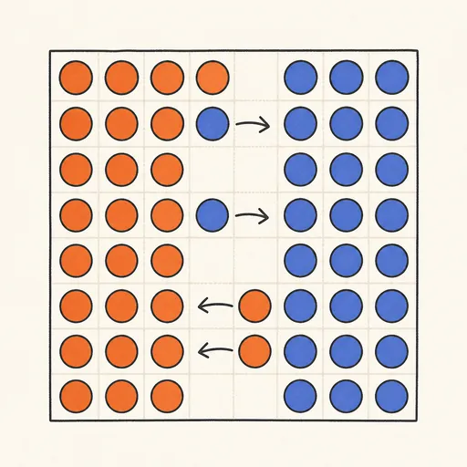
Schelling’s Segregation Model
Give agents a mild preference for similar neighbours and watch a mixed city sort itself into stark blocks.
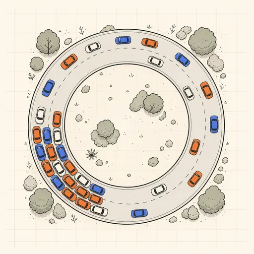
Traffic Jam Simulator
See phantom traffic jams appear from nothing on a ring road with the Nagel–Schreckenberg model.