Slope Fields, Explained
After reading this you will be able to look at a first-order differential equation, picture it as a field of little slopes, and predict where a solution curve dropped at any point will travel.
What a slope field is, in one picture
A first-order differential equation has the form y' = f(x, y). It does not tell you y directly. Instead it tells you the slope of y at every point of the plane. Feed it a location (x, y) and it hands back one number: how steeply a solution passing through that point must be rising or falling.
So take a grid of points, and at each one draw a short dash tilted to the slope that f reports there. That collection of dashes is the slope field. It is a portrait of the whole equation before you have solved anything.
Here is the hook. Take y' = y. At the point (0, 1) the slope is 1, a 45-degree dash. At (0, 2) the slope is 2, steeper. Along the whole line y = 0 every dash is flat. Trace a curve that stays tangent to the dashes starting from (0, 1) and you get y = e^x, growing faster the higher it climbs. You did not solve the equation. You read it off the wall.
When to reach for a slope field
Slope fields earn their keep when an equation is easy to evaluate but hard or impossible to solve in closed form. The equation y' = x^2 + y^2 has no elementary solution, yet its slope field is trivial to draw: at every point compute x^2 + y^2 and tilt a dash. You immediately see solutions steepening as they leave the origin.
Use a slope field when you care about qualitative behavior: Does the solution blow up? Settle to a constant? Oscillate? Which starting values head one way and which head the other? A slope field answers these before any number gets integrated.
Slope fields only work for equations you can write as y' = f(x, y), that is, first order and solved for the derivative. A second-order equation like y'' = -y needs a phase plane in two variables, not a slope field in the x-y plane. You can reduce it to a system and view that instead.
Do not use a slope field to read off precise numeric values. The dashes give you direction, not decimals. For accurate values you integrate, and even then a coarse method drifts. The companion page Euler vs Runge–Kutta shows exactly how far the cheap method wanders off the true curve.
The formula and the intuition
The dash at a grid point (x, y) has slope
Here m is the tangent of the dash's angle, f is the right-hand side of your equation, and (x, y) is the grid point. A dash of slope 2 rises two units for every one unit it runs. To draw it with fixed length L, split it into horizontal and vertical parts:
The \sqrt{1 + m^2} keeps every dash the same length no matter how steep, so a slope of 100 looks like a nearly vertical tick rather than a huge streak. That normalization is why steep regions stay readable.
To grow a solution curve through a chosen starting point, you follow the dashes. The explorer uses fourth-order Runge–Kutta (RK4), which takes a step of size h using a weighted average of four slope samples:
where k_1 = f(x_n, y_n) is the slope at the start of the step, k_2 and k_3 are slopes at the midpoint, and k_4 is the slope at the far end. Averaging four samples cancels most of the error of a single flat step. The curve is integrated both forward (increasing x) and backward (decreasing x) so it threads through your clicked point in both directions.
A worked example: the logistic equation
The demo defaults load the logistic equation, a standard model of bounded growth:
Reading the field, then integrating one curve
First read off equilibria. The slope is zero wherever y(1-y) = 0, so at y = 0 and y = 1. Those two horizontal rows of flat dashes are the constant solutions.
- Between them, say at
y = 0.5, the slope is0.5 × 0.5 = 0.25, positive, so curves rise toward1. - Above the top line, at
y = 1.5, the slope is1.5 × (-0.5) = -0.75, negative, so curves fall back toward1. - Below the bottom line, at
y = -0.5, the slope is-0.5 × 1.5 = -0.75, negative, so curves run away downward.
Now drop an initial condition at (0, 0.1) and take one RK4 step with h = 0.5.
- k_1 = f(0, 0.1) = 0.1 \times 0.9 = 0.09.
- Midpoint guess y = 0.1 + 0.25 \times 0.09 = 0.1225, so k_2 = 0.1225 \times 0.8775 \approx 0.1075.
- Refined midpoint y = 0.1 + 0.25 \times 0.1075 = 0.1269, so k_3 = 0.1269 \times 0.8731 \approx 0.1108.
- End guess y = 0.1 + 0.5 \times 0.1108 = 0.1554, so k_4 = 0.1554 \times 0.8446 \approx 0.1312.
- Combine: y_1 = 0.1 + \frac{0.5}{6}(0.09 + 2(0.1075) + 2(0.1108) + 0.1312) \approx 0.1547.
The exact logistic solution through (0, 0.1) is y = 1 / (1 + 9 e^{-x}), which at x = 0.5 gives 0.1548. The RK4 step matched it to four figures with a single step of width 0.5.
y = 1. Every logistic solution between the two equilibria has this S shape.Reading and interpreting the field
Train your eye on four features, each with a plain meaning.
- Equilibria
- Rows of horizontal dashes. These are constant solutions where f(x, y) = 0. For y' = y(1-y) they sit at
y = 0andy = 1. - Stability
- Look at the dashes just above and below an equilibrium. If they point toward it from both sides, it is stable and nearby solutions converge on it. For the logistic model
y = 1is stable andy = 0is unstable: solutions flee zero and pile up at one. - Isoclines
- Curves where the slope is constant. Setting f(x, y) = c gives the set of points with dash slope
c. Along an isocline every dash is parallel, which makes the field quick to sketch by hand. - Non-crossing
- Where f is smooth, two distinct solution curves never meet. If they touched, both would need the single slope f reports there, and they would have to continue identically. That is the uniqueness theorem drawn in dashes.
Common mistakes
The first trap is treating dashes as the curve. A dash is only tangent at its own point. A solution can bend sharply from one dash to the next when the slope changes fast, so never sketch straight through several dashes at once.
Do not integrate across an equilibrium. A curve released just below y = 1 in the logistic field approaches 1 but never reaches or crosses it, because the equilibrium is itself a solution and solutions cannot cross where f is smooth. If your numeric curve appears to jump over y = 1, your step size h is too large and RK4 overshot. Shrink h.
The second trap is forgetting that the field for an autonomous equation (no explicit x) looks the same in every vertical slice. For y' = y(1-y) the slope depends only on y, so sliding a dash left or right changes nothing. Beginners waste effort computing columns that are all identical.
The third trap is reading stability backward. Check the dashes on both sides. An equilibrium with arrows pointing in from above but out from below is not stable; it is a one-sided (semi-stable) point, and small nudges decide the outcome.
Related tools
Once a curve moves in two coupled variables you need arrows, not dashes. The Vector Field Visualizer releases particles into a full 2D field and shows divergence and curl. To watch a first-order system tumble into chaos, the Lorenz Attractor integrates three coupled equations at once.
The logistic equation here is smooth and predictable, but its discrete cousin the Logistic Map Bifurcation shatters into chaos as one parameter climbs. For the integration engine itself, compare methods on Euler vs Runge–Kutta. And to see a partial differential equation smooth a spike over time, try the Heat Equation Simulator.
Frequently asked questions
Why do solution curves never cross in a slope field?
Where f(x, y) is smooth (continuous with a bounded derivative in y), the Picard-Lindelof theorem guarantees exactly one solution through each point. Two curves crossing would demand two different curves sharing a point and slope, which the theorem forbids. Crossings can appear only where f is singular or undefined.
What is the difference between a slope field and a vector field?
A slope field draws direction only, as an undirected dash, and applies to a single equation y' = f(x, y). A vector field draws arrows with both direction and length, and describes a system with a separate rule for each coordinate. A slope field is a vector field stripped of magnitude and reduced to one dependent variable.
How accurate is the curve the explorer draws?
It uses RK4, whose error per step scales like h^5 and whose total error over an interval scales like h^4. In the worked example a single step of h = 0.5 hit the exact logistic value to four figures. Halving h cuts the accumulated error by roughly a factor of 16.
Can I use a slope field for an equation with no closed-form solution?
Yes, and that is where it shines. The field for y' = x^2 + y^2 needs only arithmetic at each grid point, even though the solution involves special functions. You see solutions steepen and blow up in finite x without ever writing them down.
Why are all the dashes the same length even when the slope is huge?
Each dash is normalized by \sqrt{1 + m^2} so its drawn length is fixed. Without that, a slope of 50 would swamp the plot. Normalization keeps steep and shallow regions equally legible while preserving the tilt that carries all the information.
Related tools
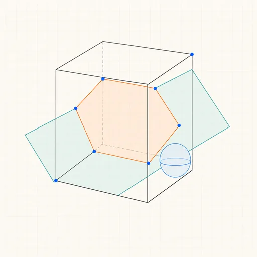
3D Geometry Board
Points, lines, planes, spheres and polyhedra on an orbiting camera — slice solids with planes, unfold nets, drop the Dandelin spheres into a cone and drag everything.
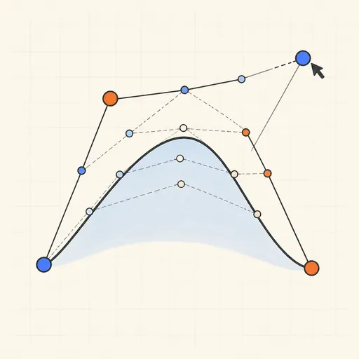
Bézier Curve Playground
Drag control points and watch De Casteljau’s algorithm construct a Bézier curve step by step.
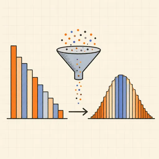
Central Limit Theorem Demo
Sample from any lopsided distribution and watch the averages pile up into a bell curve.
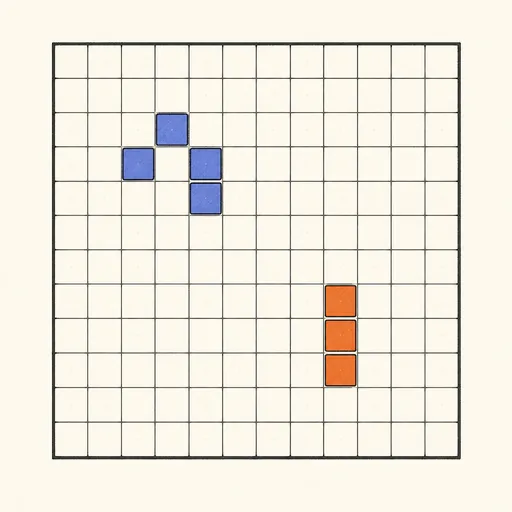
Conway’s Game of Life
Paint cells and watch Conway’s cellular automaton breed gliders, guns and oscillators.
Dynamic Geometry Board
Construct with points, lines, circles and transformations, then drag anything — the construction stays true, and a checker tells you which relations are theorems.

Fantasy Map Generator
Roll a seed and get a continent: coastlines, mountains, rivers, biomes and named towns, ready for your campaign.