PID Control, Explained
After reading this you will know what each of the three PID gains does, how to read a step response, and how to tune a loop by hand without chasing oscillations forever.
A PID controller is a feedback rule that watches the gap between what you want and what you have, then pushes an actuator to close that gap. Set a car's cruise speed to 30 m/s, and the controller reads the actual speed, computes the error, and chooses a throttle. The clever part is that it does this with just three numbers, the gains K_p, K_i and K_d, and nothing else about the car.
Here is the hook. Start the cruise control process in the simulator with pure proportional gain, say Kp = 400, and command 30 m/s. The car settles near 28.8 m/s, not 30. It stays stuck 1.2 m/s short forever. That leftover gap is the steady-state error, and no amount of extra proportional gain removes it cleanly. Add a small integral term and the car climbs to exactly 30 m/s over a few seconds. That one observation, why P alone cannot reach the target but P plus I can, is the whole intuition behind integral action.
What the controller actually computes
Define the error as setpoint minus measurement: e(t) = r(t) - y(t), where r is the reference (30 m/s) and y is the process variable (the speed you measure). The parallel-form PID controller outputs
Read the three terms physically. The proportional term K_p e reacts to the error right now: the bigger the gap, the harder the push. The integral term K_i \int e\, d\tau accumulates past error, so even a tiny persistent gap keeps growing the push until the gap is gone. The derivative term K_d\, de/dt reacts to how fast the error is changing, braking the response before it overshoots. Each term answers a different question: where am I now, how long have I been wrong, and where am I heading.
The simulator evaluates this expression every step and integrates the process (a small differential equation) with fourth-order Runge-Kutta. The three term contributions are plotted separately, so you can watch the integral term ramp up while the proportional term fades as the error shrinks.
Why integral action removes the offset
Return to the stuck cruise car. With pure proportional control the car needs some throttle u^* just to hold 30 m/s against drag. The only way a P controller produces throttle is through a nonzero error, since u = K_p e. So the error settles at exactly e^* = u^* / K_p. If holding speed needs u* = 480 and Kp = 400, then e^* = 1.2 m/s. That matches the 28.8 m/s we saw.
The integral term breaks this deadlock. It keeps adding to the output as long as any error remains, so at steady state the integral has absorbed the full 480 of throttle while the error has fallen to zero. Raising K_p to 2000 shrinks the offset to e^* = 0.24 m/s but never kills it, and high K_p brings oscillation. Integral action removes offset for a price: it adds phase lag, which means overshoot.
When to reach for PID, and when not
PID fits processes that are roughly linear, single-input single-output, and slow enough to measure and act many times per time constant. Temperature, speed, level, pressure and position loops are the classic fits. The oven process in the simulator is a good stress test because it has dead time: open the door and the sensor does not react for several seconds.
PID struggles when the process has long dead time relative to its response, strong nonlinearity, or coupled variables that fight each other. The drone hover is near the edge: it is a double integrator, so it needs real derivative action to stay stable, and pure PI will oscillate badly. For dead-time-dominated plants a predictive controller (a Smith predictor or model predictive control) beats a hand-tuned PID. Reach for PID first anyway, because it is cheap, well understood, and often good enough.
A worked tune on the demo data
Reproducing the cruise-control step
Load the tool with its field defaults (click the demo button) and command a step from 0 to 30 m/s on the cruise process. Follow the gains below and watch the response change.
- Set
Kp = 400,Ki = 0,Kd = 0. The speed rises and settles near 28.8 m/s. Steady-state error is about 1.2 m/s, exactly 480/400. - Raise to
Kp = 1200. The offset shrinks to about 0.4 m/s, but the approach now overshoots slightly and takes longer to settle. - Keep
Kp = 1200and addKi = 150. The speed now reaches exactly 30 m/s. Overshoot grows to roughly 12%, peaking near 33.6 m/s before coming back down. - Add
Kd = 180. The overshoot drops to about 4% and the loop settles faster. The derivative term produces a sharp negative spike right after the step, braking the rise.
Those four steps show the standard trade-off in miniature: P sets speed of response and leaves offset, I removes offset and adds overshoot, D removes overshoot and adds sensitivity to noise.
Reading the four numbers that matter
A step response is summarized by four metrics, all displayed live in the tool.
- Rise time
- How long the process variable takes to go from 10% to 90% of the step. In step 3 above, from 3 m/s to 27 m/s, that is roughly 3.6 seconds.
- Overshoot
- The peak above setpoint as a percentage. A peak of 33.6 m/s on a 30 m/s target is (33.6 - 30)/30 = 12\%.
- Settling time
- When the variable stays within a band (often \pm 2\%) of setpoint and never leaves. For a 30 m/s target that band is 29.4 to 30.6 m/s.
- Steady-state error
- The final gap once everything settles. With integral action this should read 0.0; without it, 1.2 m/s on the P-only case.
These fight each other. Tuning for fast rise time usually buys overshoot. Tuning for zero overshoot usually buys a sluggish rise. A common target for a well-damped loop is 5 to 10% overshoot, because that is near the fastest settling time you can reach: squeezing overshoot to 0% stretches the settling time out.
Common mistakes that make a loop misbehave
Four problems account for most failed PID loops, and each has a fix built into the simulator.
Integral windup. When the actuator saturates (full throttle, valve wide open) the error persists, so the integral keeps accumulating even though the output cannot grow. When the process finally catches up, that bloated integral drives a huge overshoot. Toggle actuator limits and anti-windup in the tool: with limits on and anti-windup off, a water-tank step can overshoot by 40% or more; turn anti-windup on and the overshoot drops back toward 10%.
Derivative kick. Taking de/dt on the error means a step change in setpoint produces an instantaneous spike, since the error jumps. The standard fix is to differentiate the measurement instead of the error, which removes the kick while keeping the damping.
Derivative noise. The derivative term amplifies high-frequency sensor noise, because differentiation multiplies a signal's amplitude by its frequency. Enable sensor noise with a large K_d and the controller output becomes a jittery mess. A first-order derivative filter tames it.
Do not copy gains from one process to another. A Kp of 1200 that tunes the cruise car nicely will send the oven into violent oscillation, because the oven's gain, time constant and dead time are completely different. Gains are specific to the plant and even to its operating point.
Using the relay auto-tuner
If you do not want to tune by hand, the auto-tuner runs an Astrom-Hagglund relay experiment. It replaces the controller with a simple on-off relay, which forces the loop into a steady oscillation at its critical frequency. From that oscillation it reads two numbers: the ultimate gain K_u (the proportional gain at the stability limit) and the ultimate period T_u (the oscillation period in seconds). The classic Ziegler-Nichols rule then sets
Here T_i and T_d are the integral and derivative times, related to the gains by K_i = K_p / T_i and K_d = K_p T_d. Suppose the relay finds K_u = 2000 and T_u = 4 s. Then K_p = 1200, T_i = 2 s so K_i = 600, and T_d = 0.5 s so K_d = 600. Ziegler-Nichols aims for a quarter-amplitude decay, which typically means 20 to 50% overshoot. Treat it as a starting point and then back off K_p or K_i if that is too aggressive.
Frequently asked questions
What is the difference between parallel and standard PID form?
The parallel form uses three independent gains K_p, K_i, K_d. The standard form writes K_p(1 + 1/(T_i s) + T_d s), using times instead of gains. They describe the same controller: K_i = K_p/T_i and K_d = K_p T_d. The simulator uses the parallel form so each slider moves one term.
Why does my loop oscillate when I increase Kp?
High proportional gain reacts so hard to error that it overshoots, then overcorrects the other way. Every process has an ultimate gain K_u above which the oscillation never dies. Stay well below it, typically at 0.6\,K_u or less, and add derivative action to damp the swing.
Can I use PI without the D term?
Yes, and most industrial loops do. The derivative term helps with fast processes and double integrators like the drone, but it amplifies noise and is often left at zero for flow and level loops. PI gives zero steady-state error with simpler, calmer behavior.
What does negative gain mean?
Some processes respond in the opposite direction: more cooling raises a temperature error you defined as setpoint minus measurement. Those need reverse action. In the simulator the process sign is already set correctly, so keep the gains positive unless the output visibly drives the error the wrong way.
Why is Ziegler-Nichols considered aggressive?
It targets quarter-amplitude decay, where each overshoot is a quarter of the previous one. That looks lively but tolerates 20 to 50% overshoot and a loop that rings for several cycles. For processes where overshoot is costly, start from the Ziegler-Nichols numbers and cut K_p by a third.
Related tools
If you want to see feedback and dynamics in other physical settings, try the Nuclear Reactor Simulator, where temperature and xenon feedback make the plant fight your control inputs. The Power Grid Simulator is a large-scale control problem: hold 50 Hz while load and generation drift. For the electrical building blocks of a controller, the Circuit Simulator lets you watch capacitors integrate and differentiate signals directly. And the Rocket Designer & Staging Lab shows what happens when an unstable plant needs active control to stay pointed the right way.
Related tools
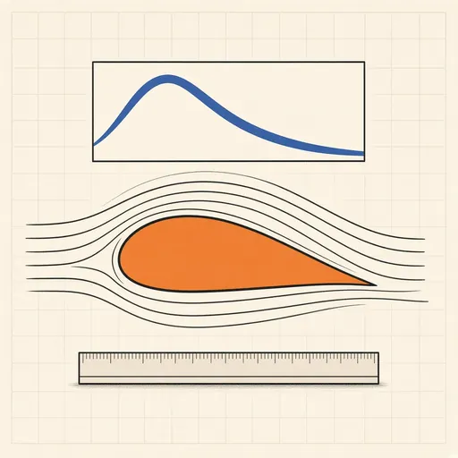
Airfoil Designer & Analyzer
Shape a NACA airfoil, see its pressure distribution and plot lift and drag polars, XFOIL-style, in the browser.

Bottle Rocket Simulator
Fill a soda-bottle water rocket, pump it up and launch it: find the water level, pressure and fins that fly highest.
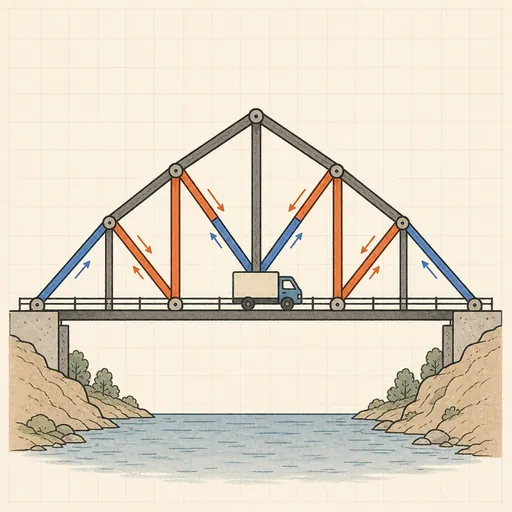
Bridge Builder & Truss Simulator
Design a truss bridge, send a truck across and watch every member strain, buckle or snap under load.
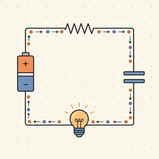
Circuit Simulator
Build analog circuits on a grid and watch current flow live — batteries, resistors, capacitors, LEDs and more.
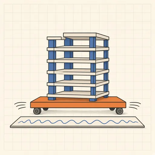
Earthquake Shake Table Simulator
Shake a multi-story building with an earthquake and watch it sway, crack or survive, with base isolation and dampers.
Gear Generator
Design involute spur gears, racks and planetary sets, watch them mesh and export SVG or DXF for laser cutting.