p-Hacking, Explained
After reading this you will know why running many statistical tests on the same noise almost guarantees a "significant" result, how to compute that risk exactly, and how to keep it in check.
What p-hacking is, with one hook
Suppose you compare two groups that come from the same source. There is no real difference between them. The true effect is exactly zero. You run a t-test and get a p-value. Do this once and you probably see a boring, large p-value like 0.42. Nothing to report.
Now run the same pointless comparison twenty times, each on a fresh pair of noise samples. At least one of those twenty tests will very likely clear the usual p < 0.05 threshold. Not because anything is real, but because you gave chance twenty attempts. Report only that one test and hide the other nineteen, and you have manufactured a false discovery. That practice, searching through many analyses until something crosses the line, is p-hacking.
The simulator makes the trick visible. Every experiment draws both groups from one distribution, so you know the answer is "no effect." It then plots the p-values and counts how often pure noise hands you a publishable-looking result.
What a p-value actually measures
A p-value answers a narrow question: if there were truly no effect, how often would you see data at least this extreme by chance alone? A p-value of 0.03 means that under the null hypothesis, results this striking or more striking occur 3% of the time.
The key fact that drives everything below is this: when the null hypothesis is true, the p-value is uniformly distributed on [0, 1]. Every value between 0 and 1 is equally likely. So the chance a single honest test lands below 0.05 is exactly 5%, the chance it lands below 0.10 is exactly 10%, and so on.
A p-value is not the probability that your hypothesis is true, and it is not the size of an effect. It is a statement about data frequency assuming no effect. A tiny p-value from a huge sample can still describe an effect too small to matter.
The formula for at least one false positive
Fix a threshold \alpha = 0.05. One test under the null has probability \alpha of a false positive, so probability 1 - \alpha of behaving. If you run k independent tests, the chance that all of them behave is (1 - \alpha)^k. The chance that at least one misfires is the complement.
Here \alpha is your per-test significance threshold (usually 0.05), k is the number of independent tests, and (1-\alpha)^k is the probability every test stays above the threshold. This quantity is called the family-wise error rate. It grows fast because you are multiplying a number slightly below 1 by itself many times.
Put numbers in. At k = 1 the risk is 0.05. At k = 5 it is 1 - 0.95^5 = 0.2262, about 23%. At k = 14 it crosses one half: 1 - 0.95^{14} = 0.5123. At k = 20 it is 1 - 0.95^{20} = 0.6415, roughly 64%. At k = 50 it reaches 1 - 0.95^{50} = 0.9231, over 92%.
1 - 0.95^k. The vertical marker sits at k = 20, where the risk is about 64%.A worked example reproducing the demo
Twenty tests on pure noise
The demo runs 20 independent tests, each comparing two groups drawn from the same standard normal distribution, at \alpha = 0.05. Here is how to read the outcome without running the code.
- Each test's p-value is a draw from the uniform distribution on [0, 1], because both groups share one source and the true difference is zero.
- The expected number of "significant" results is k \cdot \alpha = 20 \times 0.05 = 1. On average one test in twenty will falsely fire.
- The number of false positives follows a binomial distribution with n = 20 and p = 0.05. The chance of zero false positives is 0.95^{20} = 0.3585, so the chance of at least one is 1 - 0.3585 = 0.6415.
- The chance of exactly one is 20 \times 0.05 \times 0.95^{19} = 0.3774. Exactly two is \binom{20}{2} \cdot 0.05^2 \cdot 0.95^{18} = 0.1887.
So a typical run of the demo shows one red bar in the histogram, sometimes zero, sometimes two, rarely three or more. Reload it a dozen times and roughly two-thirds of the runs will show at least one red "significant" bar that means nothing.
Reading the p-value histogram
Under the null the p-values spread evenly across [0, 1]. If you bin them into ten equal buckets of width 0.1, each bucket holds about one tenth of the tests. That flatness is the signature of noise. There is no clustering near zero because nothing real is pushing p-values down.
Contrast that with a study where a real effect exists. Then the histogram leans hard toward zero: many small p-values, few large ones. So the shape of the histogram is itself a diagnostic. A flat histogram says "these tests are consistent with pure chance." A spike near zero says "something is going on." A suspicious spike just below 0.05 with a gap above it is a classic fingerprint of selective reporting.
Common mistakes that produce fake significance
P-hacking rarely looks like fraud. It usually looks like ordinary flexibility in analysis. Each choice below quietly multiplies the number of tests you ran.
- Testing many outcomes
- Measure 20 variables, report the one with
p < 0.05. That is 20 tests, so the risk of at least one false hit is 64%, not 5%. - Optional stopping
- Peek at the p-value after every few subjects and stop when it dips below
0.05. Repeated peeking is repeated testing, and it inflates the error rate well beyond 5%. - Subgroup slicing
- No overall effect, so you split by sex, age band and region until one slice reaches significance. Every slice is another test.
- Flexible exclusions
- Try the analysis with and without outliers, with several transformations, and keep the version that works. Each variant is a hidden test.
The damage comes from selective reporting. Running 20 tests is fine if you report all 20 and adjust for them. The problem is running 20 and presenting the survivor as if it were the only test you ever did.
How corrections rein it in
Two standard fixes exist. The Bonferroni correction tests each hypothesis at \alpha / k instead of \alpha. With k = 20 that means judging each test at 0.05 / 20 = 0.0025. The family-wise error rate then becomes 1 - (1 - 0.0025)^{20} = 0.0488, back under 5%. The cost is power: real but modest effects may no longer clear the stricter bar.
The false discovery rate approach, due to Benjamini and Hochberg, is less severe. Instead of guaranteeing no false positive at all, it controls the expected fraction of your "discoveries" that are false, typically at 5%. Rank the p-values, then find the largest rank i where p_{(i)} \le (i/k)\,\alpha, and declare everything up to that rank significant. This keeps more true findings when many effects are real.
The honest habit behind both methods is the same: decide your analysis before you see the data, count every test you run, and report them all.
Related tools
P-hacking is a chance phenomenon, so the site's probability toys pair with it well. The Monte Carlo Playground shows the opposite lesson, how averaging many random samples converges to a truth rather than manufacturing a lie. The Law of Large Numbers demo makes that convergence concrete. For where sampling variation itself comes from, see the Central Limit Theorem Demo and the Galton Board. The Bootstrap Resampling Visualizer builds confidence intervals honestly from one dataset, and Simpson's Paradox Visualizer shows another way statistics mislead when you slice data carelessly. If you want to feel how easily noise fools the eye, try Guess the Correlation.
Frequently asked questions
Why are p-values uniform when there is no effect?
Because the p-value is defined as the probability of a result at least as extreme as the one observed. Feeding a continuous test statistic through its own cumulative distribution always produces a uniform variable on [0, 1]. So under the null every p-value between 0 and 1 is equally likely, which is exactly why each has a 5% chance of falling below 0.05.
Is a single significant result ever trustworthy?
Yes, if it was the only planned test and the analysis was fixed in advance. A p-value near 0.001 from one pre-registered test is very different from a 0.048 plucked from 30 attempts. Trust depends on how many tests were run, not just the number you see.
Does Bonferroni ever go too far?
It can. Because it guards against even a single false positive, at large k it demands very small p-values and may miss real effects. When many hypotheses are genuinely true, false-discovery-rate control keeps more of them while still limiting the false fraction to about 5%.
How many tests do I need before it is more likely than not to find something?
Solve 1 - 0.95^k \ge 0.5. That gives k \ge \ln(0.5)/\ln(0.95) = 13.51, so at k = 14 the odds of at least one false positive first pass one half, at 0.5123.
Is p-hacking always deliberate?
No. Most of it is unconscious. Analysts try several reasonable choices, keep the one that "works," and never count the discarded attempts as tests. The fix is procedural, not moral: plan the analysis first and report every test you ran.
Related tools
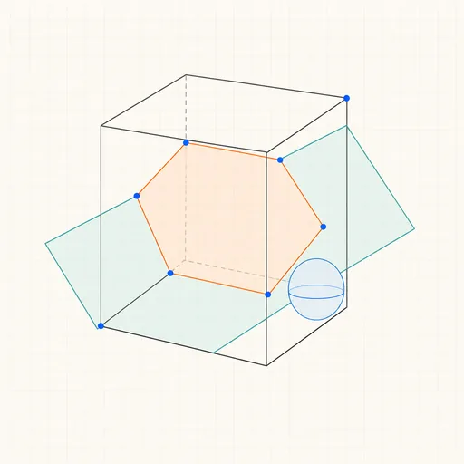
3D Geometry Board
Points, lines, planes, spheres and polyhedra on an orbiting camera — slice solids with planes, unfold nets, drop the Dandelin spheres into a cone and drag everything.
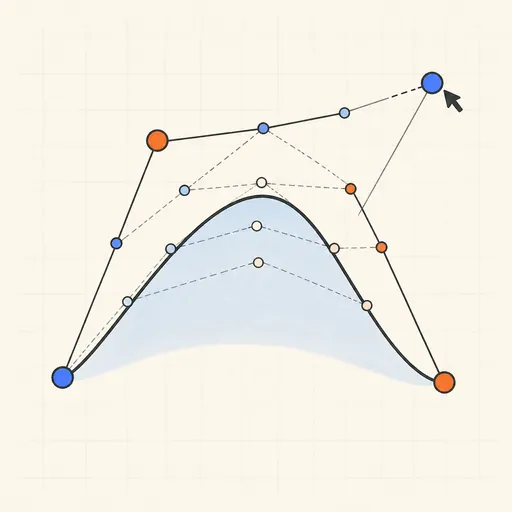
Bézier Curve Playground
Drag control points and watch De Casteljau’s algorithm construct a Bézier curve step by step.
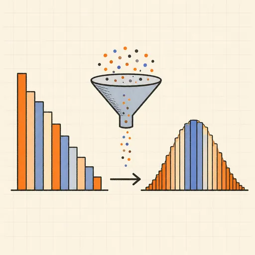
Central Limit Theorem Demo
Sample from any lopsided distribution and watch the averages pile up into a bell curve.
Conway’s Game of Life
Paint cells and watch Conway’s cellular automaton breed gliders, guns and oscillators.
Dynamic Geometry Board
Construct with points, lines, circles and transformations, then drag anything — the construction stays true, and a checker tells you which relations are theorems.

Fantasy Map Generator
Roll a seed and get a continent: coastlines, mountains, rivers, biomes and named towns, ready for your campaign.