Immune System vs Infection, Explained
After reading this you will understand the race between exponential pathogen growth and a ramping immune response, be able to write down the equations behind the simulation, and predict when the body clears an infection and when it loses.
What the model is, in one picture
Imagine a square patch of tissue. It starts full of healthy cells. You drop a single pathogen somewhere inside. That pathogen drifts around at random, and every so often it divides. When a pathogen touches a healthy cell, it infects it, and the infected cell becomes a factory for more pathogens. Left alone, the pathogen count grows roughly like P(t) = P_0 \cdot 2^{t/\tau}, doubling every \tau ticks.
The tissue is not defenseless. Immune cells patrol at some speed. Each one senses pathogens within a radius r, chases the nearest one it detects, and destroys it on contact. As the infection grows, it recruits more immune cells, so the immune count climbs too. The whole simulation is a contest between two rising curves. Catch the infection while its numbers are small and the immune cells mop it up. Fall behind the doubling and the pathogen fills the tissue first.
Here is the hook. Suppose a pathogen doubles every 12 ticks and you start with 1. After 120 ticks that is 2^{10} = 1024 pathogens. Delay the immune response by just one doubling time, 12 ticks, and the response now faces twice as many targets. That single delay is the difference between clearing and losing.
When this model helps and when it misleads
Use this simulation to build intuition about rates. It answers questions like: if the pathogen divides 30% faster, how much faster must immune cells move to compensate? What detection range is needed before recruitment even matters? These are the same questions predator-prey ecology asks, dressed in biological clothing.
Do not use it to make claims about real immunology. It has no antibodies, no memory cells, no cytokine cascade, no distinction between innate and adaptive response. The "immune cell" here is a dot that chases the nearest dot of another color. It captures the shape of the dynamics, not the mechanism.
The single most important honest limit: real immune systems have memory, so a second exposure is cleared far faster than the first. This model has no memory. Every run starts from a naive tissue. Do not read anything about vaccines or reinfection into these curves.
The equations behind the dots
Underneath the individual agents lies a well-known set of population equations. If you average over the random motion, the counts of healthy cells H, pathogens P and immune cells I follow rate equations. Pathogen growth is the first piece:
Here \beta is the infection rate: how quickly a pathogen turns a nearby healthy cell into new pathogens, so the growth term scales with both how much fuel is left (H) and how many pathogens are already present (P). The term \delta I P is destruction: each immune cell removes pathogens at rate \delta, which folds in detection range and chase speed. More immune cells, or more effective ones, means a bigger negative term.
Healthy cells only fall, as pathogens consume them:
Immune cells grow in response to the infection, then relax back when it fades:
The recruitment rate \rho says how strongly the presence of pathogens summons new immune cells. The decay rate \mu is the slow return to baseline once P drops. The key insight sits in the first equation: near the start, H is nearly full and I is nearly zero, so \frac{dP}{dt} \approx \beta H_0 P. That is exponential growth. The immune term only bites once \delta I catches up to \beta H.
The tipping point is a single inequality. The infection is cleared when the immune destruction rate exceeds the growth rate before the tissue is used up:
Explore the race yourself
A worked run using the demo defaults
Load the tool with its default values and seed one infection. To reproduce the numbers by hand, use the rate equations with \beta = 0.08, \rho = 0.01, \delta = 0.10, \mu = 0.02, starting from H_0 = 1000, P_0 = 1, I_0 = 0, with an Euler step of 1 tick.
Stepping the equations forward
- Tick 0: P = 1, I = 0. Growth term \beta H P = 0.08 \times 1000 \times 1 = 80 per tick is huge relative to P, but the tissue is barely dented.
- Early ticks: with I \approx 0, P grows fast. By tick 20, integrating step by step gives roughly P \approx 60 and I \approx 6. Destruction \delta I = 0.6 is still far below growth \beta H \approx 75.
- Crossover: recruitment keeps pushing I up. Around tick 40, I \approx 35 and H has dropped to about 550, so \delta I = 3.5 approaches \beta H = 44. Not yet, but closing.
- Peak: near tick 55, P reaches its maximum of about 300, then \delta I finally exceeds \beta H and \frac{dP}{dt} turns negative.
- Clearance: P falls back toward 0 by tick 120. With P gone, the -\mu I term slowly returns I to baseline. Final healthy count settles near 480: the infection cost about half the tissue.
Reading the three curves
Every run gives you three population curves. Read them together, not one at a time.
- Healthy cells
- Only ever falls. The final level tells you the damage done. A run that clears with 480 of 1000 healthy cells left "won" but cost half the tissue. A run that ends at 950 was a clean, early catch.
- Pathogens
- The shape that matters most. A single hump that returns to zero means clearance. A curve that flattens against the ceiling near 1000 means the pathogen won. The peak height and the peak time tell you how close the race was.
- Immune cells
- Rises with a lag, peaks after the pathogen peak, then decays. If it never gets steep enough, the infection outruns it.
Watch the gap in timing between the pathogen peak and the immune peak. A short lag means a well-matched response. A long lag, or an immune curve still climbing while pathogens hit the ceiling, is the signature of a losing run.
Common mistakes when interpreting runs
The first error is treating a single run as the truth. The agents move randomly, so two runs with identical settings can differ. A borderline case near \beta = 0.10 might clear in one run and lose in the next. Always run several times before concluding.
The second error is confusing "cleared" with "harmless." A run can clear the pathogen while destroying 60% of the tissue. In the numbers above, clearance still left healthy cells at 480 out of 1000. Survival and low damage are different outcomes.
The third error is over-tuning one parameter. Doubling immune speed helps only if detection range is large enough to find targets. Fast cells that sense nothing wander uselessly. The destruction rate \delta bundles speed and range together, and raising one while starving the other gives diminishing returns.
The fourth error is expecting a smooth threshold. Because growth is exponential, the boundary between winning and losing is sharp. A 10% change in \beta near the tipping point can flip the outcome entirely, as the shaded region in the chart above shows.
Related simulations on this site
The predator-prey race here shows up in several other agent models. If you want to see chase-and-consume dynamics with chemical signaling, the Ant Colony Pheromone Trails and Slime Mould Networks both use local sensing to steer agents. For pure population dynamics driven by chance rather than pursuit, try the Genetic Drift Simulator. To watch selection reshape a population over generations, see Evolving Creatures. And for the collective-motion side of local rules, the Boids Flocking Simulator is the classic starting point.
Frequently asked questions
Why does starting early matter so much?
Because pathogen growth is exponential. If it doubles every 12 ticks, waiting 12 ticks to respond means facing twice the numbers, and 24 ticks means four times. The immune curve rises only linearly at first, so it cannot catch a head start once the gap is large.
Can the immune response ever be too strong?
In this model, no. More destruction always clears faster with less damage. Real immune systems can over-react and harm tissue (a cytokine storm), but this caricature has no such term. Do not read damage-from-immune-response into these curves.
What single setting flips a losing run into a winning one?
Near the tipping point, lowering pathogen growth \beta is the most direct lever, since it both slows the target and preserves fuel (H). Raising recruitment \rho works too, but with a delay, because immune cells take time to accumulate.
Why do identical settings give different outcomes?
The agents drift randomly and immune cells find targets by chance encounter within their detection range. Near a threshold, that randomness decides the race. Away from the threshold, the outcome is stable across runs.
Does the tissue ever fully recover?
Not in this model. Healthy cells only decrease; there is no regrowth term. A cleared infection leaves a permanent scar in the healthy-cell count equal to whatever the pathogen consumed.
Related tools

Boids Flocking Simulator
Watch lifelike flocking emerge from three local rules with Reynolds’ boids model.

Lenia Continuous Life
Grow smooth self-organising lifeforms like the gliding Orbium in a continuous cellular automaton.

Particle Life
A few coloured species and one table of likes and dislikes — and cells, chains and chasing creatures emerge by themselves.
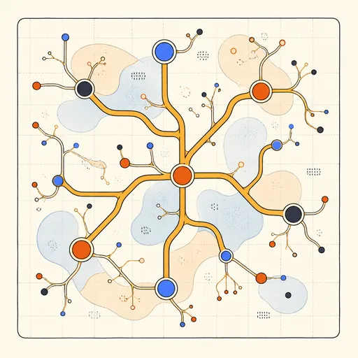
Slime Mould Networks
Watch millions of Physarum agents self-organise into living transport networks.
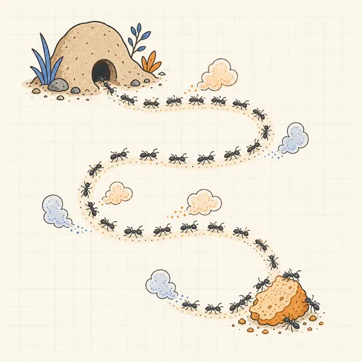
Ant Colony Pheromone Trails
Watch ants self-organise foraging highways with evaporating pheromone trails.
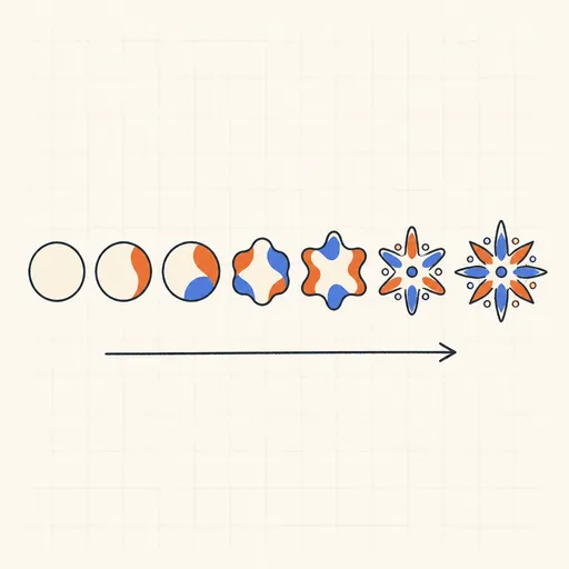
Evolving Creatures
See natural selection reshape a population of foraging creatures generation by generation.