The Galton Board, Explained

After reading this you will know why thousands of balls bouncing at random pile up into a bell curve, how to predict the shape from two numbers, and how to check the simulator's histogram against the exact binomial counts.

What the board does and why the pile is a bell curve

A Galton board is a triangular grid of pegs. You drop a ball at the top. Each time the ball hits a peg it goes left or right, and after the last row it drops into one of the bins along the bottom. The bin a ball lands in is set by one thing only: how many times it went right on the way down.

Here is the hook. Each single bounce is a coin flip, pure noise. But drop ten thousand balls and the noise cancels. Most balls take roughly as many rights as lefts, so they land near the middle. Very few take almost all rights or almost all lefts, so the edges stay short. The pile grows into a symmetric mound. That mound is the normal distribution, and it appears without anyone designing it. This is the central limit theorem made out of wood and steel.

Concretely, with r = 12 rows, a ball that goes right 6 times out of 12 lands in the center bin. The chance of exactly 6 rights is 0.2256, while the chance of 0 rights (all left) is (1/2)^{12} \approx 0.000244. The center is about 925 times more likely than the edge, which is why the pile is tall in the middle and thin at the ends.

When this model fits and when it lies

The board is a faithful picture of any sum of independent, identical yes/no events. Adding up 12 fair coin flips, counting heads in 12 dice rolls (heads meaning "rolled a 6" with p = 1/6), or tracking 12 independent shocks that push a price up or down: all of these follow the same binomial rule the board obeys.

The model stops being honest when its assumptions break. Real pegs are not perfectly fair, so a physical board often drifts slightly to one side. Real bounces are not fully independent either: a ball that leans right at one peg tends to arrive at the next peg already displaced. And the bins have finite width, so at the extreme edges balls can pile up or bounce out in ways the clean math ignores.

The formula and the intuition behind it

Let r be the number of rows (pegs deep) and p the chance of a right turn at each peg. Let k be the number of right turns, which is also the bin index counting from the left, from 0 to r. The probability a ball lands in bin k is the binomial:

The symbol \binom{r}{k} is the number of distinct paths that take exactly k rights, equal to r! / (k!\,(r-k)!). The factor p^{k}(1-p)^{r-k} is the probability of any one such path. Multiply and you get the chance of that bin.

Two summary numbers describe the pile. The mean (where the center sits) and the standard deviation (how wide it spreads):

For fair pegs, p = 0.5, so the center is at r/2 and the width is \sqrt{r}/2. When r is reasonably large, the smooth normal curve with this same \mu and \sigma traces the tops of the bars closely:

Here x is the horizontal position and e \approx 2.718. The curve peaks at x = \mu and falls off symmetrically as you move away by multiples of \sigma.

A worked example with 12 fair rows

The demo uses the field defaults: r = 12 rows and fair pegs, p = 0.5. Work out where the pile should sit before running a single ball.

Reading and interpreting the histogram

When you run the simulator, the bars will not exactly match those expected counts. They fluctuate. That scatter is the signal, not a defect. The count in each bin is itself a random number, and its typical wobble around the expected count is the square root of that count. For bin 6 with expected 2256, the wobble is about \sqrt{2256} \approx 47.5, so seeing anywhere from about 2160 to 2350 is normal.

Three things to read off the finished pile. First, the location of the peak tells you the mean, which should sit near r p. Second, the width tells you \sigma: measure how far out the bars drop to about 61% of the peak height and that distance is roughly one \sigma. Third, the symmetry tells you whether the pegs are fair. A lopsided pile means p \ne 0.5.

Compare against the overlaid normal curve. With 12 rows the match is already good; the largest gap between a bar and the curve is only a few percent of the peak. The relative fluctuation shrinks as balls accumulate: with 100 balls a bin's count wobbles by about 10% of itself, but with 10,000 balls only by about 1%. This is the same settling you see in the Law of Large Numbers demo.

Common mistakes when reading the board

The first mistake is expecting the bins to match the formula exactly. They never will. A run of 10,000 balls is a sample, and samples scatter around their expected values by roughly the square root of the count, as shown above.

The second mistake is confusing the number of bins with the number of rows. A board with r rows of pegs has r + 1 bins, indexed 0 through r. Twelve rows give thirteen bins.

The third mistake is reading a biased board as if it were fair. When p = 0.7 and r = 12, the mean shifts to 12 \times 0.7 = 8.4 and the pile becomes mildly skewed. The normal curve still fits the middle but overstates the short left tail. Skewness of a binomial is (1-2p)/\sqrt{r p (1-p)}, which for p = 0.7, r = 12 is (-0.4)/1.587 \approx -0.252: small but visible.

The fourth mistake is thinking more rows makes the pile wider in relative terms. The absolute width \sigma = \sqrt{r}/2 grows, but the number of bins grows faster, so the pile gets narrower relative to the board. With 12 rows \sigma is 15% of the bin count; with 48 rows it is 7%.

Related tools on this site

The Galton board is one physical face of a set of probability ideas you can explore elsewhere here. The Central Limit Theorem Demo lets you start from lopsided source distributions and still watch the averages pile up into a bell, generalizing what the fair board shows. To watch a single ball's path as a one-dimensional wander, see the Random Walk Explorer, since each ball's left/right sequence is exactly a random walk.

The binomial coefficients that set the bin heights are the rows of Pascal's triangle; color them by remainder in Pascal's Triangle mod n to see the Sierpinski pattern hidden inside. For other ways randomness converges on a fixed answer, try the Monte Carlo Playground and Buffon's Needle. And to feel how noise can fool you, the p-Hacking Simulator shows chance producing false signals.

Frequently asked questions

Related tools

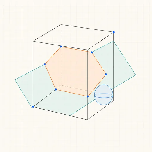
3D Geometry Board

Points, lines, planes, spheres and polyhedra on an orbiting camera — slice solids with planes, unfold nets, drop the Dandelin spheres into a cone and drag everything.

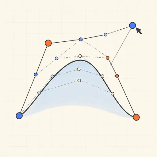
Bézier Curve Playground

Drag control points and watch De Casteljau’s algorithm construct a Bézier curve step by step.

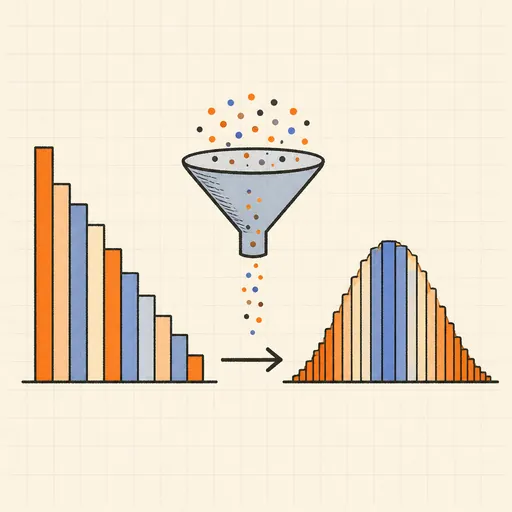
Central Limit Theorem Demo

Sample from any lopsided distribution and watch the averages pile up into a bell curve.

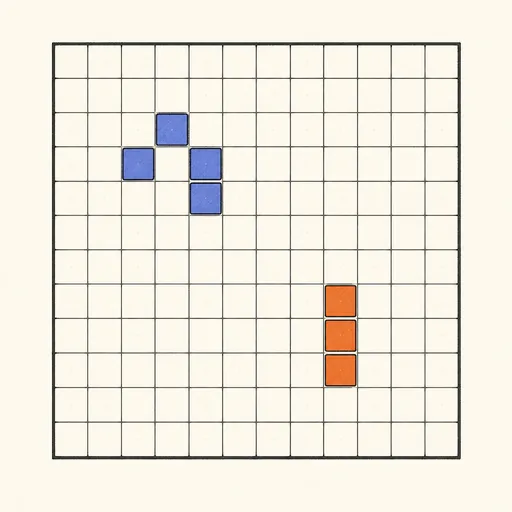
Conway’s Game of Life

Paint cells and watch Conway’s cellular automaton breed gliders, guns and oscillators.

Dynamic Geometry Board

Construct with points, lines, circles and transformations, then drag anything — the construction stays true, and a checker tells you which relations are theorems.

Fantasy Map Generator

Roll a seed and get a continent: coastlines, mountains, rivers, biomes and named towns, ready for your campaign.