Elevator Dispatch, Explained
After reading this you can predict which elevator algorithm will keep the lobby queue short during morning rush, estimate average wait time from arrival rate and car count, and spot the traffic level where any algorithm collapses.
What an elevator dispatcher actually decides
An elevator bank looks simple: cars go up, cars go down, people press buttons. The hard part is invisible. Every time someone presses a call button, a controller must decide which car answers, and in what order each car serves the calls it holds. That decision is the dispatch algorithm. Get it right and a 20-story tower moves its morning crowd with a 25-second average wait. Get it wrong and the same building leaves people stacked in the lobby for two minutes while half the cars sit idle on floor 14.
Here is the hook. Suppose 60 people arrive in the lobby over one minute, all wanting to go up. A naive controller sends the nearest car to the first person who pressed the button. That car fills, climbs, stops at eight floors, and comes back three minutes later. Meanwhile the queue behind that first person barely moved. A destination-dispatch controller instead asks each arrival for their floor before boarding, then loads car C with the six people going to floor 15, car D with the five going to floor 12, and so on. Each car now makes two or three stops instead of eight. That batching is the whole game, and this simulator lets you watch it happen.
When dispatch strategy matters, and when it does not
Dispatch strategy matters when demand is high and correlated. Morning up-peak is the worst case: almost everyone enters at the lobby and scatters to many floors, so cars fill fast and each trip must serve many stops. That is exactly where clever batching pays off.
It matters far less in light, random traffic. If one person calls a car every two minutes in a six-story building, any algorithm answers in under 20 seconds, because a car is almost always free and nearby. Spending engineering effort on dispatch there is wasted.
The single number that decides whether algorithm choice matters is the utilization: offered load divided by service capacity. Below about 0.5, all sensible algorithms look similar. Above 0.8, the gaps between them become large, and above the critical load every algorithm fails equally, just at different arrival rates.
The queueing model behind the traffic
Treat each car as a server and each waiting passenger as a customer in a queue. Passengers arrive at random. A standard model uses a Poisson arrival process with rate \lambda passengers per second. The mean gap between arrivals is 1/\lambda. If 30 people arrive per minute, then \lambda = 0.5 per second and the mean gap is 2 seconds.
Service capacity is the number of passengers the bank can deliver per second when running flat out. Let a round trip take T seconds and carry C passengers per car, with N cars. Then throughput is:
Here \mu is passengers served per second, N is car count, C is passengers carried per round trip, and T is the round-trip time in seconds. The round trip includes travel up, every stop with its door open and close, passenger transfer, and the return. The critical fact: T depends on the algorithm, because more stops per trip means a longer T and lower \mu.
The system stays stable only when arrivals stay below capacity. Define utilization \rho = \lambda / \mu. When \rho \lt 1 the queue settles to a finite length. When \rho \ge 1 the queue grows without bound: people arrive faster than any algorithm can clear them. Near the boundary, average wait explodes. A useful approximation for mean wait in a single-server-like queue is:
The 1 - \rho in the denominator is why waits shoot up as \rho climbs toward 1. At \rho = 0.5 the factor is 2. At \rho = 0.9 it is 10. At \rho = 0.95 it is 20.
How each algorithm changes the round trip
The three algorithms in this simulator differ mainly in how many stops a car makes per trip, which sets T.
- Collective control (SCAN)
- The car sweeps up answering every call in order, then sweeps down. Simple and fair. In up-peak it makes a stop at nearly every requested floor, so T is large and \mu is low.
- Nearest-car assignment
- Each new call goes to the car that can reach it soonest. This trims idle travel and cuts wait in light and medium traffic, but it does nothing to reduce stops per trip, so it still struggles in heavy up-peak.
- Destination dispatch
- Passengers enter their floor before boarding. The controller groups people by destination and loads each car with a small set of floors. Fewer stops per trip means smaller T and higher \mu. This is why it dominates tall buildings at rush hour.
A worked example from the demo defaults
A 16-floor tower, 4 cars, morning up-peak
Use the demo settings: 16 floors above the lobby, 4 cars, each holding 10 passengers, morning up-peak with 40 arrivals per minute. Car speed and door timing give a per-stop cost of about 10 seconds (accelerate, decelerate, door open, transfer, door close) and 1.5 seconds of travel per floor passed.
- Arrival rate: \lambda = 40/60 \approx 0.667 passengers per second.
- Collective control in up-peak stops at roughly 8 distinct floors per full car. Round trip: travel to the top (16 floors up and back, so 32 floor-passes at 1.5 s each = 48 s) plus 8 stops at 10 s = 80 s, total T \approx 128 s.
- Throughput: \mu = (4 \times 10) / 128 \approx 0.313 passengers per second. That is below \lambda = 0.667, so \rho \approx 2.1. The queue diverges. Collective control cannot handle this load.
- Destination dispatch groups each car to about 3 floors. Round trip: fewer stops means less travel too. Assume 24 floor-passes (12 up and back) at 1.5 s = 36 s plus 3 stops at 10 s = 30 s, total T \approx 66 s.
- Throughput: \mu = 40 / 66 \approx 0.606 passengers per second. Now \rho = 0.667 / 0.606 \approx 1.10. Still above 1, but only barely, and dropping the arrival rate to 36 per minute puts it under capacity.
The lesson from the arithmetic: nearly doubling throughput by cutting stops per trip is the difference between a lobby that clears and a lobby that fills.
Reading the histograms and queue length
The simulator shows two histograms and a queue count. Read them together.
The waiting-time histogram measures time from pressing the button to boarding a car. Watch its shape, not just its mean. A tight peak near 20 seconds is healthy. A long right tail (some people at 90 seconds while most are at 20) means the algorithm is fair on average but leaves a few passengers stranded, which is common with collective control when a car sweeps away from a waiting floor.
The time-to-destination histogram adds the ride itself. Destination dispatch often shows a slightly longer wait at the button (you wait for your assigned car) but a much shorter ride (fewer stops), so its total can win even when its wait looks worse.
Queue length is the fastest diagnostic. If the lobby count climbs steadily and never comes back down, \rho \ge 1 and no tuning of the algorithm will save you. You must add a car, raise capacity, or reduce arrivals.
Common mistakes when reading the results
Do not compare algorithms at a single low arrival rate and conclude they are equal. At 10 arrivals per minute all three finish in under 20 seconds, so the demo looks like a tie. The differences only appear near capacity. Always test at the traffic level you actually care about.
A second mistake is judging by mean wait alone. Two algorithms with the same 30-second mean can behave very differently: one delivers everyone at 30 seconds, the other delivers most at 15 seconds and a few at 120. For a real building the tail matters, because the person waiting two minutes is the one who complains.
A third mistake is forgetting that destination dispatch trades a longer button-to-board wait for a shorter ride. If you only watch the waiting histogram, destination dispatch can look worse. Check time-to-destination before deciding.
Finally, remember this is a toy model. Real controllers handle VIP floors, fire recall, staggered lunch waves, and passengers who ignore their assigned car. The simulator captures the queueing physics, not the full messy building.
Related tools on this site
Dispatch is one scheduling problem among many on this site. The Power Grid Simulator runs the same stability logic at grid scale: dispatch supply to meet stochastic demand or watch frequency collapse. The Nuclear Reactor Simulator is another control problem with a hard stability boundary, where pushing past a limit runs away fast. For a change of subject, the Circuit Simulator lets you build analog circuits and watch current flow, and the Orbital Mission Planner turns scheduling into launch-window search on a porkchop plot.
Frequently asked questions
Why does destination dispatch send me to a car across the lobby?
Because it grouped you with other passengers going near your floor. That car will make fewer stops, so even though you walk farther and may wait slightly longer to board, your ride is shorter and the whole bank moves more people per minute. The gain is at the building level, and you share in it.
Is collective control ever the right choice?
Yes. In small buildings with light traffic it is cheap, predictable, and needs no floor-entry hardware. At \rho \lt 0.5 its wait time is within a few seconds of the smart algorithms, so the extra cost of destination dispatch buys almost nothing.
What arrival rate breaks the demo building?
With the 16-floor, 4-car defaults, destination dispatch has capacity near 0.606 pax/s, or about 36 per minute. Collective control caps out near 0.313 pax/s, about 19 per minute. Set arrivals above those numbers and the matching algorithm's queue grows without bound.
Why does mean wait explode instead of rising smoothly?
The wait formula has 1 - \rho in the denominator. As \rho climbs from 0.9 to 0.95 to 0.99, that term falls from 0.1 to 0.05 to 0.01, so wait roughly doubles, then doubles again. The blow-up is built into the math of a queue near capacity, not a quirk of any one algorithm.
Does adding a car always help?
It raises capacity \mu = N C / T in proportion to N, so a fifth car in the demo lifts destination-dispatch capacity from about 0.606 to 0.758 pax/s. That drops \rho at 40 arrivals per minute from 1.10 to 0.88, moving the building from divergent to stable. Adding cars helps until shaft space or cost stops you.
Related tools
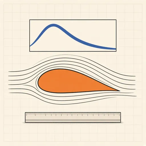
Airfoil Designer & Analyzer
Shape a NACA airfoil, see its pressure distribution and plot lift and drag polars, XFOIL-style, in the browser.
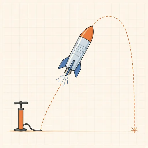
Bottle Rocket Simulator
Fill a soda-bottle water rocket, pump it up and launch it: find the water level, pressure and fins that fly highest.
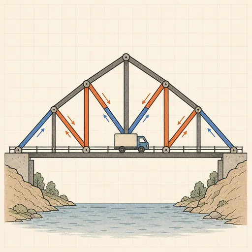
Bridge Builder & Truss Simulator
Design a truss bridge, send a truck across and watch every member strain, buckle or snap under load.
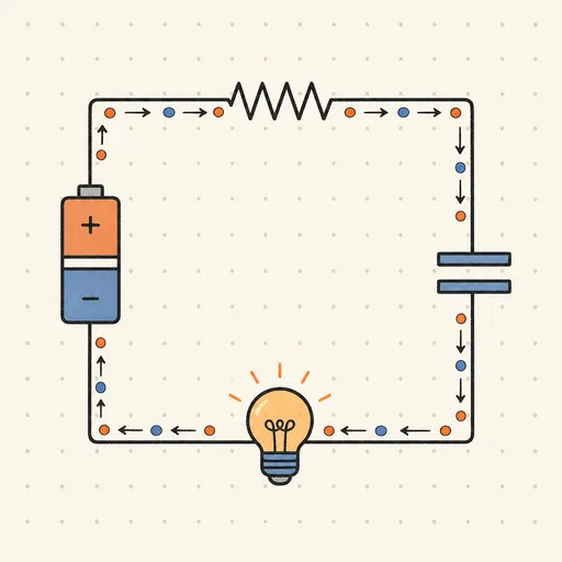
Circuit Simulator
Build analog circuits on a grid and watch current flow live — batteries, resistors, capacitors, LEDs and more.
Earthquake Shake Table Simulator
Shake a multi-story building with an earthquake and watch it sway, crack or survive, with base isolation and dampers.
Gear Generator
Design involute spur gears, racks and planetary sets, watch them mesh and export SVG or DXF for laser cutting.