Chladni Plate Patterns, Explained
After reading this you will know why sand on a vibrating square plate gathers into sharp curves, how to predict those curves from two integers m and n, and how the simulator turns a wave equation into a picture made of drifting grains.
What a Chladni figure actually is
Bow the edge of a metal plate and it vibrates. Every point on the surface moves up and down, but not by the same amount. Some points swing hard. Other points never move at all. Sprinkle fine sand over the plate and the grains bounce off the moving regions and slide until they reach the still lines. Those still lines are the pattern you see.
The still lines are called nodal lines. The regions that swing hardest are called antinodes. On a square plate driven at the right frequency, the nodal lines form clean geometric figures: crosses, grids, stars and diagonal lattices. Ernst Chladni showed this in 1787, and the shapes still carry his name.
The simulator here does not solve the full elasticity equations of a real steel plate. It uses one clean closed-form standing wave and lets thousands of grains random-walk toward the zeros of that wave. The result reproduces the classic figures faithfully while staying fast enough to run in your browser.
When this model helps and when it misleads
Use it to build intuition. If you want to see why a single number pair produces a specific symmetry, or watch one figure morph into the next as you sweep the modes, this is exactly the right toy. It makes the abstract idea of a nodal line concrete in a few seconds.
Do not use it to predict the exact pattern a physical plate will show at a given frequency. Real plates are governed by the biharmonic plate equation, their boundary is free rather than clamped, and their modes involve Bessel-like functions and edge effects that this cosine model ignores. The frequencies at which real figures appear depend on the plate material, thickness and how it is held.
The mode numbers m and n in the simulator are not frequencies in Hz. They are integer counts of half-wave arches across the plate. A real Chladni experiment maps a driving frequency to a mode; the simulator lets you pick the mode directly.
The formula and why it produces sharp lines
The plate spans the unit square, so x and y each run from 0 to 1. The vibration amplitude at each point is:
Here A(x,y) is how far the plate sits above or below rest at position (x,y), up to a sign. The integers m and n set how many arches fit along each axis. The nodal lines are the set where A(x,y) = 0. Sand collects there.
Why subtract two terms instead of using one? On a square plate the mode (m,n) and the mode (n,m) vibrate at the same frequency. Any weighted sum of the two is therefore also a valid standing wave at that frequency. The minus combination is antisymmetric under swapping x and y, so the whole diagonal y = x is automatically a nodal line. That is what gives the famous diagonal and star patterns their symmetry.
The grains do not solve A = 0 algebraically. Each grain takes a random step whose size is proportional to the local amplitude |A(x,y)|:
Here s is the vibration strength you set. Where |A| is large (an antinode), grains jump far and quickly leave. Where |A| is near zero (a nodal line), steps shrink toward nothing and grains get stuck. Over many iterations the whole population piles up on the curves A = 0. This is a physical analogy: real grains bounce off vibration, and bouncing is strongest where motion is strongest.
A worked example with the demo defaults
Predicting the pattern for the default mode
The demo button loads the field defaults. Take the representative case m = 3, n = 2 and follow the amplitude by hand.
- Write the amplitude: A = \cos(3\pi x)\cos(2\pi y) - \cos(2\pi x)\cos(3\pi y).
- Check the diagonal y = x. Then A = \cos(3\pi x)\cos(2\pi x) - \cos(2\pi x)\cos(3\pi x) = 0. The whole diagonal is a nodal line, for every x.
- Check the plate center (0.5, 0.5). Here \cos(1.5\pi) = 0 and \cos(\pi) = -1, so A = 0 \cdot (-1) - (-1) \cdot 0 = 0. The center is a node too.
- Check an off-diagonal point, say (0.25, 0.5). Then \cos(0.75\pi) \approx -0.7071, \cos(\pi) = -1, \cos(0.5\pi) = 0, \cos(1.5\pi) = 0. So A = (-0.7071)(-1) - (0)(0) = 0.7071. This is an antinode, and grains flee it.
So even before running the simulation you know two facts: the main diagonal is a nodal line, and the point one quarter across and halfway up swings hard. The finished figure shows a bright diagonal void of sand crossing a lattice of curved cells, exactly as the arithmetic predicts.
The chart below plots A along the horizontal line y = 0.5 for this mode. Every place the curve crosses zero is where sand settles along that scan line.
Explore the mode numbers
The single most instructive thing to change is the pair (m,n). Small changes rearrange the whole figure. The widget below draws the nodal lines directly from the formula so you can see the geometry without waiting for grains to settle.
Try setting m = n. The two terms become identical and cancel, so A(x,y) = 0 everywhere. There is no pattern. Always keep m \ne n.
Reading and interpreting the finished figure
Count the nodal lines and match them to the mode. As a rough guide, higher m and n give more lines and smaller cells. The number of cells scales with the product m \cdot n, so mode (5,4) looks far busier than mode (2,1).
The table below lists what to expect for a few common pairs.
| m | n | Diagonal nodal line | Approx. interior cells | Look |
|---|---|---|---|---|
| 1 | 2 | yes | 2 | simple cross-like curve |
| 3 | 2 | yes | 6 | diagonal plus lattice |
| 4 | 1 | yes | 4 | fan of arcs |
| 5 | 4 | yes | 20 | dense grid of cells |
The diagonal nodal line appears for every valid pair because of the antisymmetry noted above. If you do not see it, your grain count is too low or the vibration strength is so high that grains overshoot the thin diagonal void.
Common mistakes
Three settings spoil the figure most often.
- Equal mode numbers
- Setting m = n makes A vanish identically. The plate looks dead. Choose distinct integers.
- Vibration too strong
- If s is large, the step size stays big even near the nodes, and grains never settle. The pattern looks smeared. Lower the strength until the lines sharpen.
- Too few grains
- With only a few hundred grains the nodal lines are sparse and noisy. High modes need more grains because they have more, thinner lines to fill. A few thousand grains gives clean lines for modes up to about (6,6).
One more subtlety: the random walk finds nodal lines through a diffusion-like process, so it is stochastic. Two runs with the same settings differ slightly grain by grain, but the lines they trace are the same.
Related simulations on this site
Chladni figures are standing waves, so the closest neighbor here is the ripple tank in Wave Interference, where you can watch traveling waves add up into fixed fringes. For another take on how oscillators draw geometry, the Harmonograph traces Lissajous curves from damped pendulums, and the cosine-product structure of the Chladni formula is a close cousin of those figures.
If you want to see grains and particles respond to a field rather than to vibration, the iron filings in Magnetic Field Lines settle along field lines the way sand settles on nodes. For sensitivity and chaos instead of clean symmetry, the Double Pendulum shows how nearby starting conditions diverge.
Frequently asked questions
Why does sand collect on the still lines instead of the loud ones?
A grain sitting on an antinode gets thrown into the air with every cycle and lands somewhere new. A grain on a nodal line is not thrown, because that point does not move. So grains keep leaving loud regions and keep arriving on quiet ones. Over time the quiet lines win. The simulator models this by making step size proportional to |A|.
What is the difference between m, n and the driving frequency?
The pair (m,n) labels a mode shape: how many half-wave arches fit across the plate. A real plate reaches a given mode only when driven at that mode's resonant frequency, which depends on the plate's material and size. This simulator skips the frequency and lets you pick the mode shape directly.
Why do (m, n) and (n, m) look like mirror images?
The two orders are the same figure reflected across the diagonal y = x. Swapping m and n in the formula flips the sign of A and mirrors the coordinates, and since the pattern depends only on where A = 0, the nodal lines land in mirrored positions.
Is this how Chladni's real plates behaved?
Qualitatively yes, quantitatively no. Chladni's steel plates followed the biharmonic plate equation with free edges, giving frequencies and some fine details this cosine model does not capture. The simple product formula reproduces the visual symmetry of the classic square-plate figures, which is what makes it a good teaching model.
Can I get a completely blank plate?
Yes, by setting m = n. The two terms cancel, A = 0 everywhere, and every point counts as a node, so grains spread evenly with no pattern. It is a useful check that the formula behaves as expected.
Related tools
Buoyancy Tank
Drop blocks of different density into water and watch Archimedes decide what floats, sinks or hovers.
Double Pendulum
Swing a chaotic double pendulum and split it into a rainbow swarm to watch nearby starts diverge.
Falling-Sand Playground
Paint sand, water, oil, fire and more and watch them pour, settle, burn and react pixel by pixel.

Fluid Flow Simulator
Stir glowing dye through a real-time GPU fluid simulation.
Galaxy Collision Simulator
Smash two spiral galaxies together and watch tidal tails and bridges form.
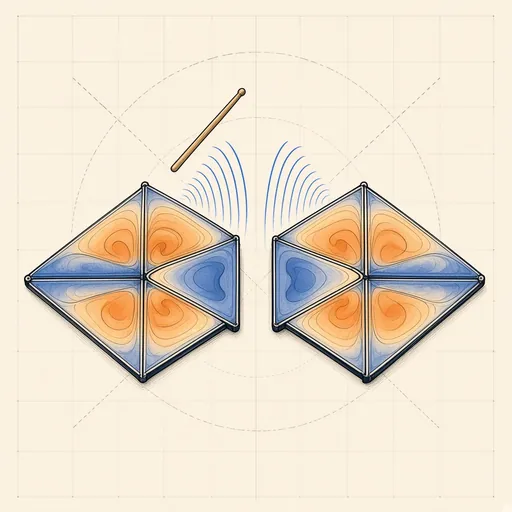
Hear the Shape of a Drum
Draw any drum and hear its true vibration modes — then meet two different drums that sound exactly the same.