The Logistic Map Bifurcation Diagram, Explained
After reading this you will be able to iterate the logistic map by hand, predict where it settles for a given growth rate, and read the fork-upon-fork structure of a bifurcation diagram without mistaking chaos for noise.
What the diagram shows
The logistic map is one line of arithmetic. Take a number x between 0 and 1, pick a growth rate r, and compute a new value:
Feed the output back in as the next input and repeat. That is the whole model. The term r x_n is unchecked growth, and the factor (1 - x_n) pulls it back down as the population crowds toward its ceiling of 1.
The surprise is what this does as you turn the single knob r. At r = 2.5 the sequence homes in on one fixed value and stays there forever. At r = 3.2 it refuses to settle on one number and instead alternates between two. At r = 3.5 it cycles through four. Past about r = 3.57 it stops repeating at all and wanders chaotically. The bifurcation diagram plots, for each r across the horizontal axis, the set of values the map settles onto on the vertical axis. Order, then splitting, then chaos, all in one picture.
When this model is useful, and when it is not
The logistic map was popularised by the ecologist Robert May in 1976 as a caricature of a population that breeds once a year, with next year's count depending only on this year's. It is a genuine teaching model for how simple feedback produces complicated behaviour. It shows, concretely, that irregular data does not require an irregular cause.
Do not read population sizes or exact dates off this map. It is a toy with one variable and one parameter, no age structure, no weather, no space. Its value is qualitative: it proves that a deterministic rule with no random input can still produce a sequence you could never predict long-term. That lesson transfers. The specific numbers do not.
Use it to build intuition about period-doubling and sensitive dependence. Do not use it to forecast anything real.
Reading the formula
Two facts about the parabola f(x) = r x (1 - x) explain everything downstream.
- Fixed point
- A value that maps to itself: x = r x (1 - x). Solving gives
x = 0and x = 1 - 1/r. The second one is the steady population you see at lowr. - Stability
- A fixed point is stable only if the slope of
fthere is smaller than 1 in size. The slope is f'(x) = r(1 - 2x). At the non-zero fixed point that works out to 2 - r.
The steady state stays stable while |2 - r| \lt 1, that is for 1 \lt r \lt 3. Exactly at r = 3 the slope reaches -1 and the fixed point loses its grip. The system cannot sit still, so it starts alternating between two values: the first period-doubling. Each later doubling happens for the same reason, applied to the two-step map, then the four-step map, and so on.
A worked example you can reproduce
The demo button uses the default sweep, r from about 2.5 to 4.0. Pick four specific values and iterate by hand from the starting seed x = 0.5. Discard the first several steps (the transient) and look at what remains.
Iterating four values of r
- r = 2.5, seed 0.5. Next values:
2.5(0.5)(0.5) = 0.625, then0.5859,0.6065,0.5966,0.6017, converging on0.6. Check: 1 - 1/2.5 = 0.6. One point. - r = 3.2, seed 0.5. After the transient the values lock into a two-cycle:
0.7995then0.5130, back and forth. Two points. - r = 3.5, seed 0.5. Settles into a four-cycle:
0.5009,0.8750,0.3828,0.8269, repeating. Four points. - r = 3.9, seed 0.5. The sequence never repeats:
0.9750,0.0951,0.3355,0.8694,0.4429, and onward with no pattern. It fills a fuzzy band. Chaos.
Those four cases are the four regimes of the whole diagram: a single value, a two-cycle, a four-cycle, and chaos. Everything else is these repeated and interleaved.
The doubling cascade and its constant
The splits do not come at even spacing. They pile up. The first doubling is at r = 3, the second at about r = 3.449, the fourth at about r = 3.544, the eighth at about r = 3.5644, and the accumulation point is r \approx 3.5699, where the period becomes infinite. Beyond that lies chaos.
Measure how much shorter each gap is than the one before. Take the ratio of successive spacings:
Here r_k is the value of r at the k-th doubling. The ratio \delta is the Feigenbaum constant. Check it with the numbers above: (3.449 - 3)/(3.544 - 3.449) = 0.449/0.095 \approx 4.73, close to 4.669 and closing in as k grows. The same 4.669 appears in many other systems approaching chaos through doubling, which is why it is called universal.
Reading and interpreting the chaotic band
The dark region past r = 3.57 is not random static. Three features are worth naming.
First, density. Where a vertical slice of the diagram looks darker, the orbit spends more of its time. The chaotic band is not uniformly grey. It has bright edges where the orbit lingers, a consequence of the parabola folding the interval onto itself.
Second, periodic windows. In the middle of the chaos, clean gaps open up. The widest sits near r = 3.83, where a stable three-cycle appears out of nowhere. By Sharkovskii's theorem, once a period-three cycle exists, cycles of every other period exist too, though most are unstable and never seen. Inside each window the doubling cascade repeats in miniature.
Third, self-similarity. Zoom into any fork and a shrunken copy of the whole diagram appears. That is the fractal signature, and it ties this one-line map to the images produced by the Mandelbrot Explorer. In fact the real slice of the Mandelbrot set corresponds directly to this bifurcation structure.
| r range | Behaviour | Points on the plot |
|---|---|---|
| 0 to 1 | Dies out to 0 | 1 (at zero) |
| 1 to 3 | Single steady value | 1 |
| 3 to 3.449 | Two-cycle | 2 |
| 3.449 to 3.544 | Four-cycle | 4 |
| 3.544 to 3.5699 | Doubling to infinity | 8, 16, 32, ... |
| 3.5699 to 4 | Chaos with periodic windows | a band, plus gaps |
Common mistakes
The first error is confusing sensitive dependence with randomness. The map is fully deterministic. Start from x = 0.5 at r = 3.9 and you get the same sequence every time. What breaks is prediction from an approximate start: at r = 3.9 two seeds differing by 0.0001 diverge to completely different values within about 15 steps, because a small error grows by a factor near e each iteration.
The second error is not discarding the transient. The first dozens of iterations still drift toward the eventual pattern. If you plot them, a clean two-cycle looks smeared. Throw away the first 100 to 200 steps before plotting, as the tool does.
To confirm a period rather than guess it, iterate far past the transient and check whether x_{n+p} equals x_n to a tolerance like 0.0001 for small p. If no small p works, you are either in chaos or in a very long window, and only a finer sweep of r tells them apart.
The third error is reading the vertical axis as a probability. It is the set of visited values, not a distribution, though the darkness of the ink does track how often each value is visited.
Related tools on this site
If the fractal repetition drew you in, the Mandelbrot Explorer shows the same iterate-and-watch idea in two dimensions, and its real axis is this diagram in disguise. For chaos in continuous time rather than discrete steps, trace the Lorenz Attractor, another deterministic system that defies long-term prediction. The Magnetic Pendulum Fractal shows sensitive dependence turned into a coloured map of outcomes.
For discrete rules that build complexity from simple updates, see Conway's Game of Life and Elementary Cellular Automata, including rule 30, whose output looks as random as the chaotic band here yet comes from three-cell arithmetic. The Chaos Game makes a fractal out of repeated random jumps, a nice contrast to the deterministic chaos above.
Frequently asked questions
Why does the population die out below r = 1?
With r < 1 the growth term r x is smaller than x itself, so each generation is smaller than the last. The only stable fixed point is 0. Try r = 0.8, seed 0.5: the sequence runs 0.2, 0.128, 0.0893, heading to zero.
What happens above r = 4?
Values escape the interval [0, 1] and shoot off to minus infinity, so the standard diagram stops at 4. At exactly r = 4 the map is fully chaotic and covers the whole interval.
Does the starting seed change the diagram?
Almost never, once the transient is discarded. For any seed strictly between 0 and 1 (excluding a measure-zero set of special points), the orbit settles onto the same attractor for a given r. The seed only changes the early transient, which you throw away.
What is period-doubling in plain terms?
It is the pattern doubling how long it takes to repeat. A fixed point repeats every step. A two-cycle repeats every two steps. Each time r crosses a threshold, that repeat length doubles: 1, 2, 4, 8, 16, and the thresholds crowd together by the factor 4.669.
Is the Feigenbaum constant special to this map?
No, and that is the point. Any smooth map with a single hump approaching chaos through doubling gives the same 4.669. It depends on the shape of the fold near its peak, not on the exact formula, which is why the constant shows up in unrelated physical systems.
Related tools
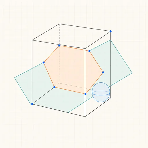
3D Geometry Board
Points, lines, planes, spheres and polyhedra on an orbiting camera — slice solids with planes, unfold nets, drop the Dandelin spheres into a cone and drag everything.
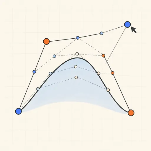
Bézier Curve Playground
Drag control points and watch De Casteljau’s algorithm construct a Bézier curve step by step.
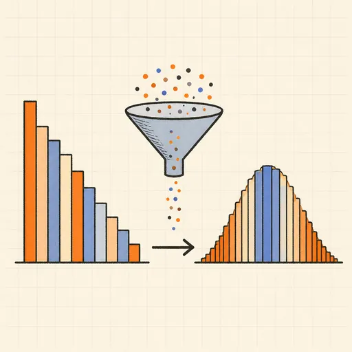
Central Limit Theorem Demo
Sample from any lopsided distribution and watch the averages pile up into a bell curve.
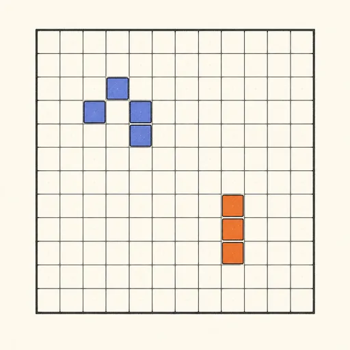
Conway’s Game of Life
Paint cells and watch Conway’s cellular automaton breed gliders, guns and oscillators.
Dynamic Geometry Board
Construct with points, lines, circles and transformations, then drag anything — the construction stays true, and a checker tells you which relations are theorems.

Fantasy Map Generator
Roll a seed and get a continent: coastlines, mountains, rivers, biomes and named towns, ready for your campaign.