Airfoil Design and Analysis, Explained
Read this and you will know how a panel method turns a wing cross-section into a lift number, how to read a pressure plot and a drag polar, and where the honest limits of an inviscid solver sit.
What an airfoil solver actually computes
An airfoil is a two-dimensional slice through a wing. Air arrives from one direction, splits at the leading edge, speeds up over the top, and rejoins at the trailing edge. Where the air goes faster the static pressure drops, and that pressure difference between the lower and upper surfaces is lift.
The tool does not simulate individual air molecules. It replaces the shape with a line of mathematical vortices along the surface, then finds the vortex strengths that make the airflow slide along the surface rather than through it. Add one more rule at the sharp trailing edge, sum up the circulation, and you get lift. This is the vortex panel method. It is the same family of method as the classic XFOIL inviscid core.
Here is the hook. Take the symmetric NACA 0012 at 4 degrees angle of attack. The solver reports a lift coefficient of about C_L \approx 0.44. Thin-airfoil theory predicts C_L = 2\pi \alpha with \alpha in radians, which gives 2\pi \times 0.0698 \approx 0.439. The panel method reproduces the textbook result to three digits because, below stall, the physics really is linear in angle.
When to use this, and when not to
Use this tool when you want the shape to lift relationship: how camber lifts the curve, how angle of attack trades lift for pressure peaks, how one section compares to another. It is fast, it runs in your browser, and it is accurate for attached flow at low Mach number.
Do not use it to predict drag with confidence, to find the exact stall angle, or to study anything after the flow separates. The solver is inviscid: it has no viscosity, so it cannot see the thin boundary layer that creates friction drag or the separation that causes stall. The drag and stall figures you see come from empirical rules bolted on afterward, not from the flow solve itself.
A pure panel method gives zero drag for any closed shape. This is d'Alembert's paradox, and it is not a bug. Any drag number here is an estimate from skin-friction and separation correlations layered on top of the inviscid pressure field. Treat it as a guide to trends, not a wind-tunnel measurement.
If you want drag and separation from an actual fluid solve, draw your shape into the Wind Tunnel (CFD Sandbox) and measure it there. For the structure that carries the wing loads, the Bridge Builder & Truss Simulator shows how members strain under load.
The geometry: four digits that draw a wing
A NACA 4-digit section is built from three numbers. The first digit is maximum camber as a percent of chord. The second is the position of that camber as tenths of chord. The last two are maximum thickness as a percent of chord. So 2412 means 2 percent camber at 40 percent chord, 12 percent thick.
The thickness is a fixed polynomial laid symmetrically about a mean camber line:
Here x runs from 0 at the leading edge to 1 at the trailing edge, t is the thickness fraction (0.12 for a 12 percent section), and y_t is the half-thickness. The camber line y_c is two parabola arcs that meet at the camber position, and the final surface points are the thickness draped perpendicular to that camber line.
The solver then resamples the surface with cosine spacing: points cluster near the leading and trailing edges where the curvature and pressure change fastest. With 160 panels, that clustering gives the leading-edge suction peak far more resolution than evenly spaced points would.
From panels to lift: the vortex method
Each panel carries a linearly varying sheet of vorticity. The unknowns are the vortex strengths \gamma_i at the panel nodes. Two conditions pin them down. First, the flow must be tangent to the surface at every panel midpoint (no air passes through the skin). Second, the Kutta condition forces the flow to leave the sharp trailing edge smoothly, which fixes the overall circulation.
Once the \gamma_i are solved from a linear system, lift follows from the Kutta-Joukowski theorem. Total circulation \Gamma is the integral of the vortex strength around the section, and in coefficient form the lift is:
where V_\infty is the freestream speed and c is the chord. The pressure at each panel comes from Bernoulli, expressed as the pressure coefficient:
Where the local speed exceeds the freestream, C_p goes negative (suction). At a true stagnation point the local speed is zero and C_p = 1. The area between the upper and lower C_p curves, integrated along the chord, is the lift again. Two routes, one answer.
Reproducing the demo: NACA 2412 at 4 degrees
The demo button loads the defaults: a NACA 2412, angle of attack 4 degrees, Reynolds number 1,000,000, Mach near 0. Walk the numbers.
- The symmetric part contributes the thin-airfoil slope: 2\pi \times \alpha = 2\pi \times 0.0698 = 0.439.
- The 2 percent camber adds a zero-angle lift. For 4-digit camber the zero-lift angle is roughly \alpha_{L=0} \approx -2.1^\circ, so the effective angle is 4 - (-2.1) = 6.1^\circ = 0.106 rad.
- Lift becomes 2\pi \times 0.106 \approx 0.67. The panel method, which accounts for finite thickness, returns about C_L \approx 0.65.
- The moment about the quarter chord stays near C_m \approx -0.05, the signature nose-down pitch of a cambered section.
- The drag estimate at this Reynolds number lands near C_d \approx 0.006, giving a lift-to-drag ratio around 0.65 / 0.006 \approx 108, which is optimistic because the inviscid pressure drag is missing. A real 2412 near this point sits closer to 70.
The point of the exercise: lift you can trust to a few percent, drag you should read as a ballpark.
Reading the pressure plot and the polars
The pressure plot is drawn upside down by convention: suction (negative C_p) points up. The tall spike near the leading edge on the upper surface is the suction peak. As you raise the angle of attack, that peak grows sharper and taller. When it gets steep enough that a real boundary layer could not follow it, the airfoil is near stall. The inviscid solver happily draws an ever-taller peak past that point, which is exactly where it stops being physical.
The lift curve is C_L against angle. Below stall it is a straight line of slope about 0.11 per degree (that is 2\pi per radian). The drag polar plots C_L against C_d: a sideways bucket whose nose points left at minimum drag. The best lift-to-drag ratio is the point where a line from the origin just touches the polar.
To read the zero-lift angle straight off the lift curve, find where the line crosses C_L = 0. For the 2412 above it crosses near -2^\circ. A symmetric 0012 crosses at exactly 0 degrees because it makes no lift when pointed straight into the wind.
Explore: how camber shifts the whole lift curve
Camber does one clean thing to the lift curve: it slides it left and up without changing the slope. Thickness, by contrast, barely moves lift but softens the stall and adds a little drag. Move the sliders and watch the line translate.
Common mistakes
Three errors show up again and again when people first use a panel tool.
- Trusting drag and stall as if they came from the solve
- They do not. The inviscid flow has no drag and never separates. The drag polar and stall angle are correlations. Use them for ranking shapes, not for sizing a propeller.
- Pushing the angle of attack past stall and believing the lift
- Above the stall angle the straight lift line is a fiction. A real wing at 20 degrees makes far less lift than 0.11 \times 20 would suggest, because the flow has detached.
- Ignoring Mach and Reynolds number
- At Mach above about 0.3 air compresses and the incompressible C_p is wrong; a Prandtl-Glauert correction scales it by 1/\sqrt{1 - M^2}. At Mach 0.5 that is a 15 percent boost. Reynolds number sets the drag estimate and the stall angle; a model wing at Re = 10^5 behaves very differently from an airliner at Re = 10^7.
Where this fits with the other simulators
An airfoil is one link in a longer chain. The Wind Tunnel (CFD Sandbox) solves the viscous flow this tool cannot, so it is the natural next step when you need real drag. If you are building the aircraft that carries the wing, the Rocket Designer & Staging Lab handles powered flight and staging, and the Orbital Mission Planner takes over once you are out of the atmosphere. For control of the resulting vehicle, the PID Controller Simulator lets you tune the feedback loop that holds an attitude.
Frequently asked questions
Why does a symmetric airfoil have a lift slope of 2 pi?
Thin-airfoil theory shows that for small angles the circulation grows in direct proportion to angle, and the constant works out to 2\pi per radian, about 0.11 per degree. The panel method reproduces this because it solves the same inviscid equations. Real airfoils fall a little short, typically 0.10 to 0.11 per degree, due to the boundary layer.
Can I load a real airfoil instead of a NACA shape?
Yes. Paste coordinates in Selig .dat format from any airfoil database. The solver repanels them with cosine spacing and runs the same analysis. You can also export a shape as a .dat file or as an SVG rib template at a chosen chord length.
Why is my drag number lower than published wind-tunnel data?
Because the pressure drag from separation and wake is missing. The estimate here covers skin friction and a rough separation penalty, but it cannot capture the full viscous loss. Expect the tool to read optimistic, often by 20 to 40 percent at moderate lift.
What does the quarter-chord moment coefficient tell me?
It measures the nose-up or nose-down pitching tendency about the point 25 percent back from the leading edge. A cambered section like the 2412 sits near C_m \approx -0.05, a steady nose-down pitch that the tail must trim out. A symmetric section reads near zero.
Does increasing thickness always cost performance?
No. Thickness adds a small amount of drag but gives a gentler, more forgiving stall and far more room for a strong spar. An 18 percent section is draggier than a 9 percent one at cruise, yet it stalls more gently and is easier to build stiff. The trade depends on your mission.
Related tools
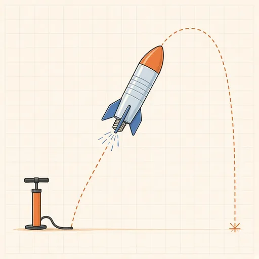
Bottle Rocket Simulator
Fill a soda-bottle water rocket, pump it up and launch it: find the water level, pressure and fins that fly highest.
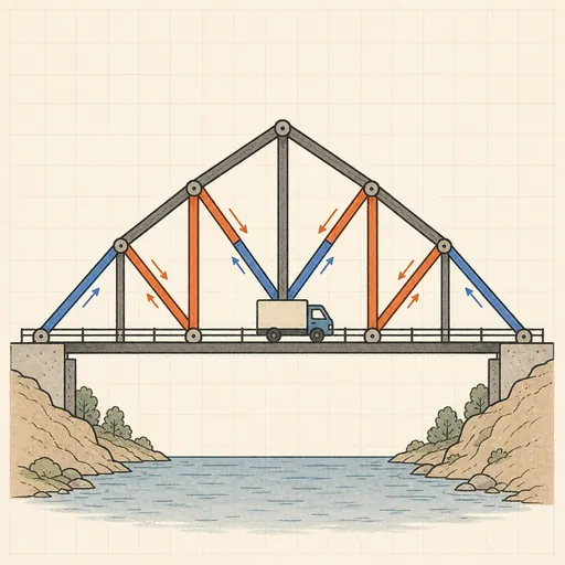
Bridge Builder & Truss Simulator
Design a truss bridge, send a truck across and watch every member strain, buckle or snap under load.
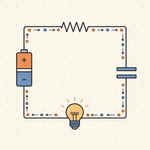
Circuit Simulator
Build analog circuits on a grid and watch current flow live — batteries, resistors, capacitors, LEDs and more.
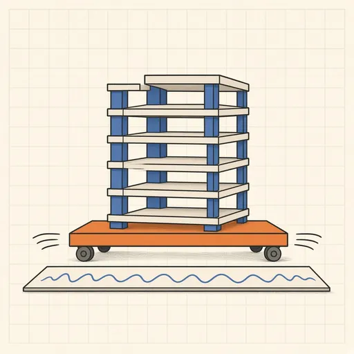
Earthquake Shake Table Simulator
Shake a multi-story building with an earthquake and watch it sway, crack or survive, with base isolation and dampers.
Gear Generator
Design involute spur gears, racks and planetary sets, watch them mesh and export SVG or DXF for laser cutting.
Nuclear Reactor Simulator
Run a pressurized-water reactor: pull control rods, manage xenon and temperature — or SCRAM before it overheats.