Wind Tunnel and CFD, Explained
After reading this you can put a shape into a virtual wind tunnel, read its drag and lift the way an aerodynamicist does, predict when a smooth wake breaks into a vortex street, and know which numbers to trust.
What a wind tunnel measures, and one example
Air flows past a shape. The shape pushes on the air, and the air pushes back. That push has two parts you care about: the force along the flow (drag) and the force across it (lift). A wind tunnel exists to measure those two forces without flying anything.
Here is the hook. Drop a plain cylinder into a slow flow and the streamlines close neatly behind it, like water rejoining after a rock. Raise the wind speed and something changes: the wake starts to shed swirls, first from one side, then the other, in a steady beat. That beat is the von Kármán vortex street. It is the same physics that makes a flag flap, a power line hum, and a tall chimney need spiral strakes to stay still. The simulation lets you watch that transition happen and read the drag climbing as it does.
The solver here is a lattice-Boltzmann method on a 2D grid. Instead of solving the Navier-Stokes equations directly, it tracks packets of fictitious particles that stream to neighboring cells and collide. Viscous fluid behavior emerges from those simple rules. That is a real technique used in engineering CFD, not a cartoon.
When to use it, and when not to
Use it to build intuition and to compare shapes. Which airfoil sheds less drag? Does rounding the back of a car help more than sharpening the front? At what speed does the wake go unsteady? These are questions about trends, and the trends this sandbox shows are physical.
Do not use it to certify a design. The grid is coarse, the flow is 2D, and a real wing lives in 3D where tip vortices and spanwise flow change the numbers. Treat a drag coefficient of 0.9 here as "high, roughly bluff-body high," not as a value you would hand to a manufacturer.
A 2D cylinder and a 3D sphere are different animals. Textbook drag coefficients you find online for a sphere (around 0.47) will not match a 2D cylinder in this tool (around 1.0 to 1.2 at moderate Reynolds number). Compare like with like.
The numbers behind the flow
Two dimensionless groups govern almost everything you see. The first is the Reynolds number, the ratio of inertial forces to viscous forces:
Here \rho is fluid density, U is the free-stream speed, L is a characteristic length (the diameter of your cylinder), \mu is dynamic viscosity, and \nu = \mu/\rho is kinematic viscosity. Low Re means syrup-like, smooth, laminar flow. High Re means the wake wants to break up.
The forces are reported as coefficients so they do not depend on how big your shape is or how fast the wind blows. Drag and lift coefficients are:
F_D is the drag force, F_L is the lift force, and the term \tfrac{1}{2}\rho U^2 is the dynamic pressure of the flow. In 2D the reference area is just the length L (per unit depth). The solver gets F_D and F_L the honest way: it sums the momentum exchanged between fluid and obstacle at every boundary cell, then divides.
The vortex street has its own clock, set by the Strouhal number:
f is the shedding frequency in hertz. For a cylinder over a wide range of Re (roughly 200 to 200000), St sits near 0.2. So if you know the speed and diameter, you can predict how often vortices peel off, and the lift signal will oscillate at that frequency.
A worked example with the default cylinder
Predicting drag and shedding for the demo cylinder
Load the demo. It places a cylinder in the flow at the default speed. Take these grid-scaled values as the setup: diameter L = 40 lattice units, free-stream speed U = 0.1 lattice units per step, kinematic viscosity \nu = 0.02.
- Reynolds number: Re = \frac{U L}{\nu} = \frac{0.1 \times 40}{0.02} = 200. That is squarely in the vortex-street range.
- Expected drag coefficient: at Re = 200 a 2D cylinder runs near C_D \approx 1.3. The gauge should read in that neighborhood, wobbling slightly as vortices shed.
- Shedding frequency from Strouhal: f = \frac{St \cdot U}{L} = \frac{0.2 \times 0.1}{40} = 0.0005 per step. That is one shed cycle every
2000steps. - Lift coefficient: the mean is near
0by symmetry, but it oscillates. Peak amplitude near Re = 200 is roughly C_L \approx \pm 0.6. Watch the lift gauge swing between about+0.6and-0.6at the frequency above.
So the story is: a steady drag around 1.3, a lift that averages to zero but rocks back and forth, and a wake that pulses once every 2000 steps. If you slow the wind so that Re drops below about 47, the shedding stops entirely and the wake becomes two fixed standing eddies.
Explore the transition yourself
Reading and interpreting the gauges
The drag gauge is your headline number. Lower is better for a car or an airfoil at cruise. A streamlined airfoil at a small angle can reach C_D near 0.05 in 2D, while a flat plate held broadside sits near 2.0. That is a factor of forty. Shape matters more than anything else you can change.
The lift gauge is the sideways force. For a symmetric shape at zero angle it averages zero. Tilt an airfoil and lift climbs almost linearly with angle of attack, then collapses when the flow separates: that collapse is stall. Watch for lift rising, peaking, then dropping as you increase the tilt.
The vorticity view colors the flow by how fast it is spinning locally. Vorticity is the curl of the velocity field:
u and v are the horizontal and vertical velocity components. Red and blue patches of opposite \omega alternating down the wake are the vortex street made visible. The smoke lines show where fluid goes; the vorticity view shows where it spins. Both matter.
Common mistakes
The errors below trip up almost everyone the first time.
- Reading the instantaneous drag as "the" drag
- When the wake sheds, drag oscillates. Report the time average over several shedding cycles, not one lucky snapshot. At Re = 200 that means averaging over at least
4000to6000steps. - Expecting steady flow at high speed
- If the numbers refuse to settle, the flow is genuinely unsteady, not broken. Above the shedding threshold there is no steady answer. That is the physics.
- Comparing to 3D coefficients
- Every reference value in this article is 2D. A 3D body relieves pressure around its edges and usually has lower drag. Do not mix the two.
- Drawing a shape with sharp interior gaps
- Thin slots and one-cell-wide spikes are smaller than the grid can resolve. The solver will do something, but it will not be trustworthy. Keep features several cells wide.
- Ignoring the walls
- If your shape fills most of the tunnel height, the walls squeeze the flow and inflate drag. This is called blockage. Keep the shape well under half the tunnel height for clean numbers.
To get a clean drag reading, let the simulation run until the drag gauge settles into a repeating pattern, then eyeball the midpoint of its swing. That midpoint is your time-averaged C_D.
Related simulators on this site
If you like watching physical laws play out on a grid, several other sandboxes here run the same way. The Bridge Builder & Truss Simulator shows forces flowing through structure instead of fluid, and it pairs naturally with this tool: the vortex street you see here is exactly the load that shakes a real bridge. For fields of a different kind, the Circuit Simulator lets you watch current spread through a network. If large-scale physics is your interest, the Rocket Designer & Staging Lab and the Orbital Mission Planner both trade fluids for gravity and thrust.
Frequently asked questions
Why is my drag coefficient not matching the textbook value exactly?
Two reasons. The grid is coarse, so it smooths sharp gradients and can miss a few percent of the true drag. And this is 2D flow, while most textbook values you find are 3D. Expect the right trend and the right order of magnitude, not four matching digits.
What Reynolds number makes the vortex street appear?
For a cylinder, alternating shedding switches on near Re = 47. Below that you get two fixed eddies (from about Re = 5 to 47) or smooth attached flow (below Re = 5). Raise the wind speed in the tool to cross that threshold and watch the wake come alive.
Why does the lift oscillate around zero for a symmetric shape?
Vortices shed alternately from the top and bottom. Each vortex leaves a low-pressure patch that pulls the shape toward that side, so the sideways force flips sign every half cycle. The average is zero, but the swings are real and they are what make structures vibrate.
Can I trust the exact numbers for engineering?
No. Use the tool for intuition, comparison and teaching. For a design that will fly or carry load, you need a fine 3D solver and a physical wind tunnel. The footnote on the tool page says this plainly: trends and patterns are physical, exact coefficients are not wind-tunnel-grade.
What is the drag crisis I have read about?
Near Re = 300000 the thin layer of air hugging a smooth cylinder or sphere turns turbulent. Counterintuitively, that turbulent layer sticks to the surface longer, the wake narrows, and drag drops sharply, from about 1.2 to 0.3. It is why golf balls have dimples. A browser-scale 2D solver will not reach that regime, but the drag curve above shows where it lives.
Related tools
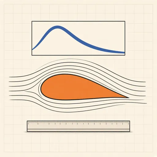
Airfoil Designer & Analyzer
Shape a NACA airfoil, see its pressure distribution and plot lift and drag polars, XFOIL-style, in the browser.
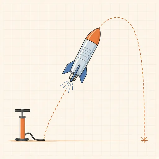
Bottle Rocket Simulator
Fill a soda-bottle water rocket, pump it up and launch it: find the water level, pressure and fins that fly highest.
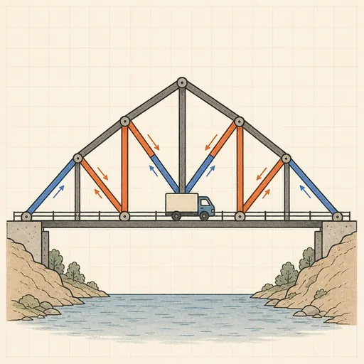
Bridge Builder & Truss Simulator
Design a truss bridge, send a truck across and watch every member strain, buckle or snap under load.
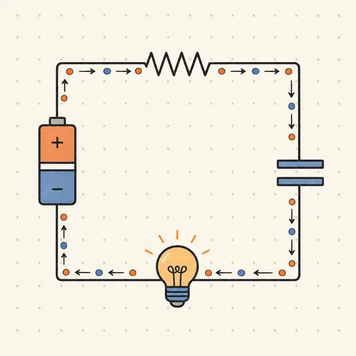
Circuit Simulator
Build analog circuits on a grid and watch current flow live — batteries, resistors, capacitors, LEDs and more.
Earthquake Shake Table Simulator
Shake a multi-story building with an earthquake and watch it sway, crack or survive, with base isolation and dampers.
Gear Generator
Design involute spur gears, racks and planetary sets, watch them mesh and export SVG or DXF for laser cutting.