Sugarscape, Explained
After reading this you will understand how a few greedy foraging rules produce a lopsided wealth distribution, how to measure that inequality with a Gini coefficient, and how to read the Sugarscape simulator without over-reading it.
What Sugarscape is
Sugarscape is an agent-based model built by Joshua Epstein and Robert Axtell in their 1996 book Growing Artificial Societies. The world is a grid of cells. Each cell holds some sugar and has a maximum capacity. Sugar regrows over time. Agents sit on the grid, look around, move to the richest cell they can reach, eat the sugar there, and burn a fixed amount of sugar each step to stay alive. An agent whose sugar store hits zero dies.
No agent trades, saves strategically, or plans ahead. Every agent runs the same one-line rule. Yet after a few hundred steps the population sorts itself into a small group of rich agents and a large group of poor ones. The wealth histogram is not bell-shaped and symmetric. It is skewed hard to the right: many agents near the bottom, a long thin tail of high wealth. That skew is the hook. It looks like the wealth curves economists measure in real societies, and it comes out of rules that contain no notion of class, luck, or policy.
The point of the model is not that it predicts any real economy. The point is existence: it shows that a highly unequal distribution can emerge from identical simple rules and small starting differences, with no central design and no unfairness written into the code.
When to use it, and when not to
Reach for Sugarscape when you want to see how macro-scale structure grows out of micro-scale rules. It is a teaching model for emergence: inequality, spatial clustering, carrying capacity, and boom-and-collapse of a foraging population. It pairs well with other emergence models on this site, such as Schelling's Segregation Model, where a mild individual preference produces stark city-wide sorting.
Do not use it to forecast real inequality or to argue that any specific policy will or will not work. The map has no jobs, no inheritance law, no education, and no money. Its variables (vision, metabolism, sugar) are stand-ins, not measured quantities. Treat a Gini value from the simulator as a fact about the model, not about the United States or anywhere else. For dynamics driven by explicit differential equations rather than grid rules, see the Predator–Prey Simulator and the SIR Epidemic Simulator.
The rules and the numbers behind them
Two rules run the whole thing. The first governs the land. Each cell has current sugar s and capacity c. Every step the sugar grows back:
Here \alpha is the regrowth rate, the fixed amount of sugar each cell recovers per step, and c is the cell's ceiling. A rich peak might have c = 4; a poor valley c = 1. Larger \alpha means the land refills faster, which feeds more agents.
The second rule governs each agent. An agent has vision v (how many cells it can see along each axis), metabolism m (sugar burned per step), and a sugar store w. Each step it looks at the cells within range, picks the unoccupied one with the most sugar (ties broken by nearest), moves there, and eats. Its wealth updates as:
Here g_t is the sugar harvested from the chosen cell this step. If w_{t+1} \le 0 the agent dies and is removed. So survival needs the long-run harvest to keep pace with metabolism. An agent with vision v = 6 sees more candidate cells than one with v = 1, so it more often finds a full cell. An agent with metabolism m = 1 outlasts one with m = 4 on the same food. Those two differences, plus the luck of where an agent starts, are enough to split the population.
Measuring inequality with the Gini coefficient
To turn a wealth histogram into one number, Sugarscape uses the Gini coefficient. It ranges from 0 (everyone has exactly the same wealth) to 1 (one agent holds everything). A clean way to compute it for a population of n agents with wealths w_i is the mean absolute difference form:
Here |w_i - w_j| is the wealth gap between agents i and j, the double sum adds up every pairwise gap, and \bar{w} is the mean wealth. Dividing by 2 n^2 \bar{w} scales the result to the 0 to 1 range. A real economy measured on income sits roughly between 0.25 and 0.60; Sugarscape often lands in the same band, which is why the shape feels familiar.
A five-agent Gini by hand
Take five surviving agents with wealths 2, 3, 5, 10, and 30. Work the formula step by step.
- Mean wealth: \bar{w} = (2+3+5+10+30)/5 = 10.
- Sum of all pairwise absolute differences. The distinct pairs give: |2-3|=1, |2-5|=3, |2-10|=8, |2-30|=28, |3-5|=2, |3-10|=7, |3-30|=27, |5-10|=5, |5-30|=25, |10-30|=20. That sums to 126.
- The double sum counts each pair twice and the zero self-pairs add nothing, so \sum\sum |w_i - w_j| = 2 \times 126 = 252.
- Denominator: 2 n^2 \bar{w} = 2 \times 25 \times 10 = 500.
- Gini: G = 252 / 500 = 0.504.
A Gini of 0.504 is steeply unequal. Notice the single agent holding 30 drives it: drop that agent to 10 and the mean falls to 6, the pairwise sum falls to 2 \times 46 = 92, and the Gini drops to 92 / (2 \times 25 \times 6) = 0.307. One rich outlier moves the number a lot.
Reproducing the demo and reading the histogram
Run the simulator with the default settings from the demo button. Sugar grows on two rich peaks and thins out into valleys. Agents crowd onto the peaks, valleys empty, and after a few hundred steps the wealth histogram settles into a stable right-skewed shape even as individual agents keep dying and the survivors keep foraging. The chart below shows a representative final distribution: most agents cluster at low wealth, a thin tail reaches high.
The number to watch alongside the histogram is the Gini coefficient. Early on, when agents start with similar small stores, the Gini is low, near 0.1. As foraging plays out, well-placed high-vision, low-metabolism agents accumulate while others starve, and the Gini climbs and then levels off. The next chart shows a typical trajectory.
Common mistakes when reading the model
The most frequent error is treating the Gini as a measured social fact. It is a property of a toy grid. A second error is comparing runs with different starting populations without noticing that population size changes the outcome. Start 400 agents on a landscape that can feed 180, and the extra 220 mostly starve in the first 60 steps, which spikes early inequality before it settles. Start 150 agents on the same land and few die, so the early Gini stays low.
A single very rich agent can swing the Gini by 0.1 or more, as the worked example showed. Do not read tiny differences between runs as meaningful. Run the same settings several times and compare the spread, not one number.
A third mistake is confusing cause and effect between vision and wealth. High vision correlates with survival, but so does starting on a peak. Because the two compound, you cannot say vision alone made an agent rich. That confound is the point: small advantages multiply, and after 400 steps the winners look far apart even though they began nearly equal.
Related simulations on this site
If Sugarscape's emergence interests you, three neighbors explore the same theme with different mechanics. The Traffic Jam Simulator shows a jam forming from nothing on a ring road, another macro pattern from local rules. The Forest Fire Model balances tree growth against lightning strikes into a self-organised critical state. For population dynamics driven by explicit equations rather than grid foraging, the predator-prey and SIR simulators linked earlier are the natural next stops.
Frequently asked questions
Why does inequality appear if all agents follow the same rule?
Because the agents are not born into the same conditions. Vision and metabolism differ slightly, and starting position matters even more: an agent placed on a rich peak eats well from step one, while an agent in a valley starts behind. These small gaps compound step after step, and the greedy rule rewards whoever is already ahead. A Gini near 0.47 emerges without any rule that favors the rich.
Does a faster regrowth rate reduce inequality?
Usually yes, within the model. When the land refills faster, more cells are full when an agent arrives, so more agents survive and fewer are pushed to zero. The interactive widget shows the Gini falling from about 0.45 at regrowth 1 to about 0.25 at regrowth 4, because the poor bins fill in as scarcity eases.
Is a Gini of 0.47 realistic?
It sits in the same range as many real income Ginis, which run roughly 0.25 to 0.60. That resemblance is why the model is famous. It does not mean the model measures any real economy. The match is structural, not quantitative.
What happens if I start with too many agents?
The population overshoots what the land can feed, then crashes as the surplus starves. The survivor count settles near the landscape's carrying capacity regardless of how many you started with, so 400 agents and 250 agents on the same map often end near the same final population.
Can agents ever escape poverty in this model?
Rarely, once the distribution has settled. A poor agent needs to reach richer cells before its store hits zero, but the rich cells are crowded by agents who got there first. There is no trading, no saving strategy, and no help, so mobility is low. That rigidity is a consequence of the bare rules, not a design choice.
Related tools
Gerrymandering Sandbox
Draw the districts yourself and watch the same voters produce opposite election results.
Pareto Frontier Evolution
Watch a genetic algorithm breed bridge designs and trace out the weight-vs-stiffness Pareto frontier, generation by generation.
SIR Epidemic Simulator
Watch an epidemic spread and burn out with the classic susceptible–infected–recovered model.

Sailing & Tacking Simulator
Sail a boat against the wind — trim to the polar diagram, ride the shifts and race the optimal route.
Schelling’s Segregation Model
Give agents a mild preference for similar neighbours and watch a mixed city sort itself into stark blocks.
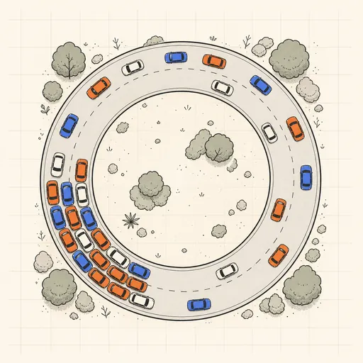
Traffic Jam Simulator
See phantom traffic jams appear from nothing on a ring road with the Nagel–Schreckenberg model.