The Heat Equation, Explained
After reading this you will be able to predict how a temperature profile on a rod smooths and decays, run the finite-difference update by hand, and read the glowing temperature map for what it tells you about diffusion.
What the simulator shows
Put a hot spot in the middle of a cold metal rod and let it sit. Within a moment the sharp peak slumps into a rounded bell, the bell widens, and the whole rod slides toward a uniform temperature. This simulator runs that process live in one dimension, with the two ends held cold at zero.
The rule behind the motion is short: each point drifts toward the average of its two neighbours. A point that is hotter than the average around it cools; a point that is cooler than its surroundings warms. Repeat that thousands of times per second and you get diffusion. Nothing in the rule pushes heat toward any particular shape. The bell curve appears on its own because averaging destroys sharp features first and gentle features last.
Here is the hook. Take an initial hot spot 2 units tall and about 10 grid cells wide. After a short run it is roughly 1 unit tall and 20 cells wide: half the height, twice the spread. The area under the curve stayed almost constant while the peak flattened. That trade, height for width, is the visual signature of diffusion.
When this model applies and when it does not
The 1D heat equation is a good description of temperature in a thin rod, insulated along its sides, where heat only flows left and right. It also describes the concentration of a dye spreading in a still tube, and the probability cloud of a diffusing particle. Any process where a quantity flows down its own gradient, from high to low, at a rate set by the local curvature, obeys the same equation.
It does not describe waves. A plucked string obeys u_{tt} = c^2 u_{xx}, with a second time derivative, so energy sloshes back and forth forever. The heat equation has a first time derivative, so it only relaxes and never oscillates. If you want the wave version, see the Fourier series builder for how oscillating modes stack. It also fails when the material properties change fast, when heat is generated inside the rod, or when the ends are not held fixed. Those cases need extra terms this toy does not include.
The heat equation is the exact continuous limit of a random walk. If a particle steps left or right with equal chance, the probability of finding it at position x after time t spreads exactly like temperature. Diffusion and drunken wandering are the same mathematics seen from two directions.
The equation and why it means averaging
Here u(x,t) is temperature at position x and time t. The term u_t is how fast temperature changes in time. The term u_{xx} is the second spatial derivative, the curvature of the profile. The constant \alpha \gt 0 is the diffusivity, which sets the overall speed.
Curvature is the key. Where the profile bends downward like a hilltop, u_{xx} is negative, so u_t is negative and the point cools. Where it bends upward like a valley, u_{xx} is positive and the point warms. Straight sections have zero curvature and do not change. A flat rod is the only steady shape, which is why everything drifts toward flat.
To run this on a computer, replace the derivatives with differences on a grid of spacing \Delta x and time step \Delta t. The curvature at cell i becomes the discrete second difference, and the update is:
The bracket is exactly "neighbour average minus me, doubled". If r is small, each step nudges every cell a little toward its neighbours. The single number r controls both speed and stability. Keep r \le 0.5 or the simulation blows up, a point covered below.
Reproducing the demo: a hot spot on a 5-cell rod
Use a tiny rod so the arithmetic is checkable by hand. Take 7 cells indexed 0 to 6. Cells 0 and 6 are the fixed cold ends held at 0. Start with a hot spot: u = [0, 0, 0, 4, 0, 0, 0]. Set r = 0.25, which is safely below the stability limit.
- Step 1, cell 3:
4 + 0.25(0 + 0 - 8) = 4 - 2 = 2. Its neighbours cells 2 and 4 each get0 + 0.25(4 + 0 - 0) = 1. New profile:[0, 0, 1, 2, 1, 0, 0]. - Step 2, cell 3:
2 + 0.25(1 + 1 - 4) = 2 - 0.5 = 1.5. Cell 2:1 + 0.25(0 + 2 - 2) = 1. Cell 4 by symmetry is also1. Cell 1:0 + 0.25(0 + 1 - 0) = 0.25. New profile:[0, 0.25, 1, 1.5, 1, 0.25, 0]. - Step 3, cell 3:
1.5 + 0.25(1 + 1 - 3) = 1.5 - 0.25 = 1.25. The peak keeps sinking while the shoulders keep filling.
Track the total heat, the sum of all cells. Start: 4. After step 1: 0 + 0 + 1 + 2 + 1 + 0 + 0 = 4. After step 2: 0.25 + 1 + 1.5 + 1 + 0.25 = 4. The interior conserves heat exactly; loss happens only through the cold ends, and here the ends have not yet warmed enough to bleed much away. The peak fell from 4 to 2 to 1.5 to 1.25 while the profile widened. Height for width, again.
Why sharp features die first
Break any starting profile into sine waves (its Fourier modes). A mode with wavenumber k looks like \sin(kx). Plug it into the heat equation and each mode decays on its own, independently of the others:
The decay rate is \alpha k^2. High k means fine wiggles, and because k is squared, those wiggles vanish fast. Double the wavenumber and the decay rate quadruples. A ripple with 10 times the wavenumber of a broad bump decays 100 times faster.
Concretely, take \alpha = 1. A mode with k = 1 falls to e^{-1} \approx 0.368 of its start after t = 1. A mode with k = 4 falls to e^{-16} \approx 1.1 \times 10^{-7} in the same time, effectively gone. That is why a sharp step edge blurs almost instantly while the overall hump lingers. The heat equation is a low-pass filter: it keeps smooth, broad structure and erases the crisp detail.
Reading the temperature map and the march to equilibrium
The glowing map stacks the rod's profile over time, brightest where hottest. Read it top to bottom as a history. A hot spot shows a bright core that fades and fans outward into a widening triangle of dimmer glow. A sharp step shows a crisp boundary at the top that softens into a smooth gradient within a few rows, then washes out entirely.
With cold ends fixed at zero, the only equilibrium is a flat rod at zero everywhere. Every initial condition, however dramatic, ends there. The interesting content is all in the transient: how fast, in what order, and through which shapes the profile relaxes. Two competing hot spots merge into a single broad bump before both fade, because once their tails overlap the valley between them fills in faster than the peaks can hold.
To compare runs fairly, watch the peak height, not the map's brightness. Height falls roughly as 1/\sqrt{t} for a spreading spot, and the width grows as \sqrt{t}. If you double the elapsed time and the width grows by a factor near 1.41, the simulator is behaving.
Common mistakes
The first trap is instability. If you push the time step too high so that r \gt 0.5, the explicit update overshoots. A cell corrects past the neighbour average, the error flips sign and grows each step, and the profile erupts into a jagged sawtooth that doubles in size every step. At r = 0.51 you may not notice for a while; at r = 0.6 the rod explodes in a handful of steps. Keep r at or below 0.5, and for smooth results stay near 0.25.
The second trap is confusing decay with heat loss. Interior heat is conserved; it only leaves through the ends. Early on, the peak drops sharply even though almost no heat has escaped, because the heat is spreading sideways, not vanishing. Watch the running sum to tell spreading from loss.
The third trap is expecting motion. Diffusion has no momentum. Unlike a wave, a bump never travels as a bump, and two spots never pass through each other. They only ever smear and merge. If you see something propagating cleanly, you are looking at a wave model, not this one.
Related tools
Diffusion sits inside a web of related ideas on this site. The random walk explorer shows the microscopic picture whose average is this equation. The slope field explorer and the Euler vs Runge-Kutta comparison cover the numerical methods for ordinary differential equations that the same finite-difference thinking extends. For the wave counterpart with oscillating modes, build them by hand in the Fourier epicycles tool. And for a very different rule where neighbours interact discretely rather than by averaging, compare Conway's Game of Life and the elementary cellular automata, where sharp local rules build structure instead of erasing it.
Frequently asked questions
Why does a hot spot always turn into a bell curve?
Because the solution from a single point source is exactly a Gaussian: u \propto e^{-x^2 / (4\alpha t)} / \sqrt{t}. Any narrow start looks like a point source once it spreads, so the bell shape is the universal intermediate state before the ends drain it to zero.
What does the diffusivity alpha do?
It rescales time. Doubling \alpha makes every process happen twice as fast; a shape that takes t = 2 to relax at \alpha = 1 takes t = 1 at \alpha = 2. It changes the clock, not the shapes.
Why must r stay at or below one half?
The explicit update mixes each cell with a fraction 2r of the difference to its neighbours. If 2r exceeds 1, a cell overshoots the average and the correction grows instead of shrinking. The threshold r = 0.5 is where the growth factor of the worst mode hits 1; above it, that mode explodes.
Does the rod ever reach a temperature other than zero?
Not with both ends held cold. Zero everywhere is the only steady state. If instead you held the ends at fixed nonzero values, the equilibrium would be a straight line between them, since a line has zero curvature and so never changes.
Is this the same equation used in finance and image blurring?
Yes, structurally. The Black-Scholes equation is a heat equation after a change of variables, and a Gaussian blur on an image is one step of 2D diffusion. All three erase fine detail while preserving broad structure, because all three are governed by curvature-driven smoothing.
Related tools
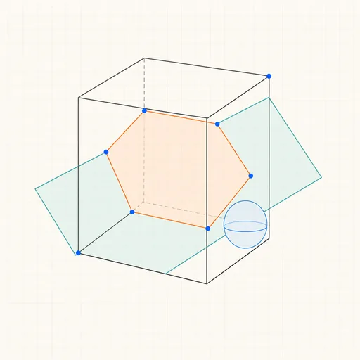
3D Geometry Board
Points, lines, planes, spheres and polyhedra on an orbiting camera — slice solids with planes, unfold nets, drop the Dandelin spheres into a cone and drag everything.
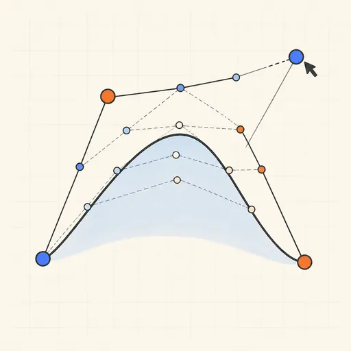
Bézier Curve Playground
Drag control points and watch De Casteljau’s algorithm construct a Bézier curve step by step.
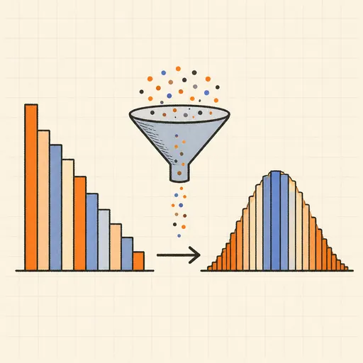
Central Limit Theorem Demo
Sample from any lopsided distribution and watch the averages pile up into a bell curve.
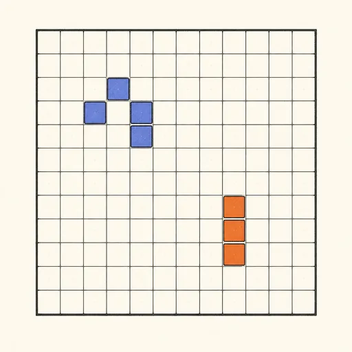
Conway’s Game of Life
Paint cells and watch Conway’s cellular automaton breed gliders, guns and oscillators.
Dynamic Geometry Board
Construct with points, lines, circles and transformations, then drag anything — the construction stays true, and a checker tells you which relations are theorems.
Fantasy Map Generator
Roll a seed and get a continent: coastlines, mountains, rivers, biomes and named towns, ready for your campaign.