The Harmonograph, Explained
After reading this you will know how four damped pendulums turn into a glowing curve, how to predict whether that curve closes or drifts, and how to pick frequencies and detune that draw the figure you want.
A harmonograph is a mechanical drawing machine. Two or more pendulums swing at slightly different rates. One carries a pen, the others move the paper, and the pen traces the combined motion. As friction bleeds energy away, the swings shrink and the curve spirals inward. The tool at /sim/harmonograph/ reproduces this by computing each coordinate as a sum of two decaying sine waves and drawing the path point by point.
Here is the hook. Set the x and y frequencies both near 2 and 3, add a whisper of detune, and the pen draws a rounded three-lobed loop. Then run it again with the ratio nudged from exactly 3:2 to 3.01:2. The single clean loop becomes a woven net, because each pass lands a little rotated from the last. Nothing changed but a hundredth of a cycle per second, yet the whole character of the drawing flipped.
What the machine actually computes
Each axis is the sum of two damped sinusoids. The classic four-pendulum harmonograph gives you two contributions to the horizontal motion and two to the vertical. Writing it out for one axis:
Here a_1, a_2 are the amplitudes (how wide each pendulum swings), f_1, f_2 are the two horizontal frequencies in radians or cycles per second, \varphi_1, \varphi_2 are the starting phases, and d is the damping rate. The factor e^{-d t} is the friction: it multiplies both terms by a number that starts at 1 and shrinks toward 0. The vertical coordinate y(t) follows the same form with its own frequencies and phases.
The two frequencies on each axis are not identical. The detune slides them apart. If the base frequency is f and the detune is \delta, the twin frequencies become f - \delta and f + \delta. With \delta = 0 the two sines lock together and you get a pure Lissajous figure. With a small \delta the figure precesses.
When to reach for it, and when not
Use the harmonograph when you want to see how two independent linear oscillators combine, and how a rational frequency ratio makes a closed curve while an irrational or slightly detuned ratio does not. It is the cleanest picture of Lissajous geometry you can get without an oscilloscope. It is also a good demonstration of damping as a pure multiplicative envelope.
Do not use it as a model of a chaotic or nonlinear system. Every term here is a plain sine wave, so the motion is completely predictable for all time. There is no sensitivity to initial conditions, no mixing, no strange attractor. If you want genuine chaos, the Double Pendulum is the right tool: it uses the full nonlinear equations, and two nearby starts diverge. The harmonograph only looks intricate.
Real Victorian harmonographs from the 1840s, usually credited to Hugh Blackburn, drew whatever their pendulum lengths happened to give. This tool lets you set the ratio exactly, which real hardware could only approximate by trial and error with adjustable weights.
Why the ratio decides everything
Ignore damping for a moment and set the detune to zero, so each axis is a single sine. Then x(t) = \sin(f_x t) and y(t) = \sin(f_y t + \varphi). The path repeats exactly when both sines return to the same phase at the same time. That happens after a time T such that both f_x T and f_y T are whole numbers of cycles.
Here p and q are the smallest whole numbers that make the ratio work. A ratio of 3/2 closes after 3 x-cycles and 2 y-cycles. A ratio of 3.01/2 is 301/200 in lowest terms, so it needs 301 x-cycles before it closes. Long before that, damping has shrunk the curve to nothing. That is why a tiny detune never closes in practice: it just weaves.
The tool reports the current frequency ratio live so you can read p{:}q directly. Simple ratios like 1:1, 2:1, 3:2 give clean, few-lobed figures. Ratios with large numerator and denominator give dense tangles.
Reproducing the demo defaults
Load the tool and press the demo button, which uses the field defaults. Suppose those defaults give f_x = 3, f_y = 2, detune \delta = 0.01, phases \varphi_x = 0 and \varphi_y = \pi/2, damping d = 0.02, and unit amplitudes. Follow the numbers.
- The horizontal twin frequencies are
3 - 0.01 = 2.99and3 + 0.01 = 3.01. The vertical twins are1.99and2.01. - At t = 0 the envelope e^{-d t} equals
1. Aftert = 50seconds it equals e^{-0.02 \cdot 50} = e^{-1} \approx 0.368. The swing is down to about 37 percent of its start. - The reported ratio is close to 3:2, so the base figure is a three-by-two loop.
- The
0.01detune means the two horizontal sines drift apart by one full cycle after 1/(2\delta) = 1/0.02 = 50 seconds. That slow drift is what rotates each pass. - By the time the figure has precessed noticeably, around
t = 50, the amplitude is already near 0.37, so the net shading fades as it rotates. That fade is the signature harmonograph look.
The envelope, in numbers
The damping factor is worth its own table because it controls how many passes you see before the pen effectively stops. The half-life of the swing (time to fall to half amplitude) is t_{1/2} = \ln(2)/d \approx 0.693/d.
| Damping d | Half-life (s) | Amplitude at t=30 | Amplitude at t=100 |
|---|---|---|---|
| 0.005 | 138.6 | 0.8607 | 0.6065 |
| 0.02 | 34.66 | 0.5488 | 0.1353 |
| 0.05 | 13.86 | 0.2231 | 0.006738 |
| 0.1 | 6.931 | 0.04979 | 0.0000454 |
Read the last row: with d = 0.1 the swing is already under 5 percent of its start by t = 30, so you get a short spiral and little weaving. With d = 0.005 the pen is still at 61 percent by t = 100, so it draws many overlapping passes and a dense net.
Reading a finished figure
Three features tell you the settings that produced a drawing.
- Lobe count
- Count the outermost bumps horizontally and vertically. Three across and two up means a ratio near 3:2. This reads the frequency ratio straight off the paper.
- Net density
- A tight woven mesh means low damping and nonzero detune, so many passes stacked with slight rotation. A single clean line means near-zero detune or heavy damping.
- Spiral rate
- How fast the curve collapses to the center measures the damping. A figure that fills the frame evenly has low d; one that shrinks fast has high d.
The phases mostly rotate and skew the figure rather than change its topology. Setting \varphi_y = \pi/2 against \varphi_x = 0 at a 1:1 ratio turns a diagonal line into a circle, the standard Lissajous demonstration.
Common mistakes
Setting the detune high while expecting a closed figure. A detune of 0.05 shifts the twin frequencies by 0.1 apart, so they never lock, and no ratio produces a clean loop. If you want a crisp closed curve, set detune to 0 and use a simple ratio like 2:1 or 3:2.
A second trap is confusing frequency ratio with frequency size. Doubling both frequencies to 6 and 4 keeps the ratio at 3:2, so the figure shape is identical; only the drawing speed changes. What matters for the picture is the ratio, not the absolute values.
A third trap is cranking damping to draw faster. High d does not speed the pen, it shrinks the swing, so you get a stubby spiral that never develops the net. To see rich weaving, keep damping low (say 0.005 to 0.02) and give it time.
Related tools
If you like combining waves, the Wave Interference tool shows the same superposition principle in two spatial dimensions, where sine sources add into fringes. The Chladni Plate Patterns tool shows standing waves on a plate, another place where frequency ratios pick out clean geometric figures. For motion that genuinely will not repeat, try the Double Pendulum and compare its chaos to the harmonograph's perfect predictability.
Frequently asked questions
Why does my harmonograph figure never close?
Either your ratio reduces to large integers, or your detune is nonzero. A ratio like 3.01:2 is 301:200, which needs 301 x-cycles to close, far more than damping allows. Set detune to 0 and pick a simple ratio to get a closed curve.
What does the detune slider actually do?
It splits each axis into two sines at f - \delta and f + \delta. Those two slowly drift apart, beating once every 1/(2\delta) seconds. That slow beat rotates each pass of the figure, which is the woven net you see in real drawings.
Is this the same math as Lissajous figures?
Yes, with zero damping and zero detune. Each axis becomes a single sine, and the pair traces a Lissajous curve that closes whenever the frequency ratio is rational. Damping adds the inward spiral; detune adds the precession.
Does higher damping make the pen move faster?
No. Damping only shrinks the amplitude through the factor e^{-d t}. The frequencies set the speed. Raising damping just ends the drawing sooner with a smaller figure.
How long should I let a figure run?
Long enough for the amplitude to fall near zero. With d = 0.02 the swing is at 13.5 percent by t = 100, so a run to about 100 to 150 seconds of simulated time captures nearly the whole figure.
Related tools
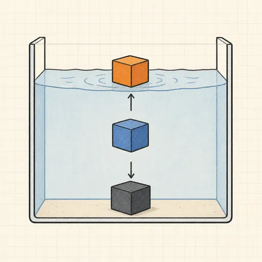
Buoyancy Tank
Drop blocks of different density into water and watch Archimedes decide what floats, sinks or hovers.
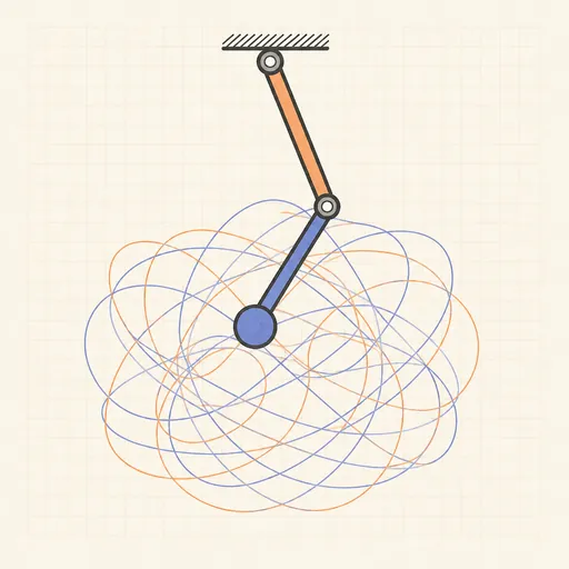
Double Pendulum
Swing a chaotic double pendulum and split it into a rainbow swarm to watch nearby starts diverge.
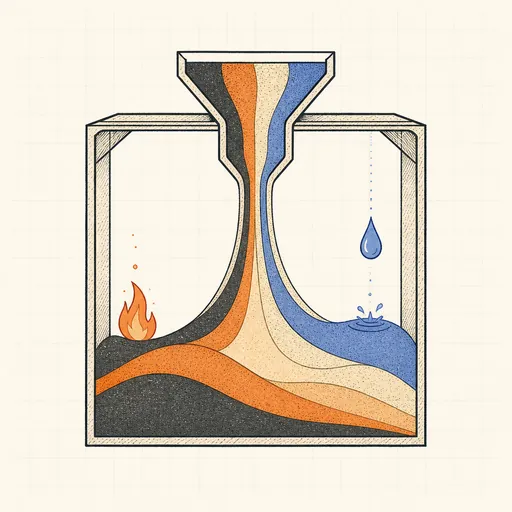
Falling-Sand Playground
Paint sand, water, oil, fire and more and watch them pour, settle, burn and react pixel by pixel.
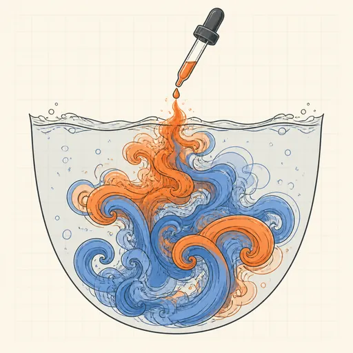
Fluid Flow Simulator
Stir glowing dye through a real-time GPU fluid simulation.
Galaxy Collision Simulator
Smash two spiral galaxies together and watch tidal tails and bridges form.
Hear the Shape of a Drum
Draw any drum and hear its true vibration modes — then meet two different drums that sound exactly the same.