Euler vs Runge–Kutta, Explained
After reading this you can predict how far a numerical ODE solver will drift from the true answer, tell an O(h) method from an O(h⁴) one by watching the error shrink, and choose a step size that buys accuracy without wasting work.
What these methods do
A differential equation gives you the slope of a curve at every point, but not the curve itself. Numerical solvers rebuild the curve by walking along it: start at a known point, ask the equation for the slope, take a small step, repeat. The only information a solver ever receives is slope values from the function f(t, y). How it uses those slopes decides everything.
Euler's method is the simplest possible walk. It reads one slope, follows it in a straight line for a step of length h, and repeats. Runge-Kutta of order 4 (RK4) reads four slopes per step, at cleverly chosen points, and blends them. Both are cheap and run entirely in your browser. But on the same problem with the same step size, their accuracy differs by a factor you can watch grow.
Take the test equation y' = y with y(0) = 1, whose exact solution is y(t) = e^t. At t = 1 the truth is 2.71828. With step size h = 0.25, Euler reaches 2.4414, an error of 0.277. RK4 reaches 2.71825, an error of 0.0000282. Same equation, same coarse step, error smaller by about 9800 times.
When to use each
Use Euler when you want to understand a method, sketch a rough trajectory, or teach the idea of stepping along a slope. It is one line of arithmetic and it is honest about what integration means. Do not trust it for quantitative work: to get three correct digits you often need thousands of tiny steps.
Use RK4 as the sensible default for smooth, non-stiff problems. It costs four function evaluations per step instead of one, but its error falls so fast that a coarse RK4 step usually beats a fine Euler step both in accuracy and in total work. In the example above, RK4 with h = 0.25 (4 steps, 16 evaluations) crushes Euler with h = 0.25 (4 steps, 4 evaluations) and would still beat Euler with h = 0.0001 (10000 steps).
Neither method is a good choice for stiff equations, where some components decay far faster than others. There an explicit method must take absurdly small steps just to stay stable, no matter how accurate it is in principle. Implicit solvers (backward Euler, BDF, implicit Runge-Kutta) are built for that case.
The formulas and the intuition
Euler takes the current slope and assumes it holds for the whole step:
Here y_n is the current estimate, h is the step size, and f(t_n, y_n) is the slope the equation reports at the current point. The trouble is that the true slope changes across the step, so a single reading at the start is systematically wrong when the solution curves.
RK4 fixes this by sampling four slopes and taking a weighted average:
The four slopes are k_1 = f(t_n, y_n) at the start, k_2 = f(t_n + h/2,\, y_n + \tfrac{h}{2}k_1) and k_3 = f(t_n + h/2,\, y_n + \tfrac{h}{2}k_2) at the midpoint, and k_4 = f(t_n + h,\, y_n + h k_3) at the end. The midpoint slopes get double weight. This weighting is not arbitrary: it is tuned so that the step matches the Taylor expansion of the true solution through the h^4 term, which is why the error per step scales like h^5 and the accumulated error like h^4.
The headline rule follows from those exponents. Euler's global error is O(h): halve h and the error roughly halves. RK4's global error is O(h^4): halve h and the error drops by a factor of 2^4 = 16.
A worked example on y' = y
One Euler step and one RK4 step, h = 0.25
Start at t_0 = 0, y_0 = 1, with f(t, y) = y.
- Euler slope: f = y_0 = 1. Step: y_1 = 1 + 0.25 \cdot 1 = 1.25. The truth at
t = 0.25is1.28403, so Euler already trails by0.03403. - RK4 slope 1: k_1 = 1.
- RK4 slope 2: k_2 = y_0 + \tfrac{0.25}{2}(1) = 1.125.
- RK4 slope 3: k_3 = y_0 + \tfrac{0.25}{2}(1.125) = 1.140625.
- RK4 slope 4: k_4 = y_0 + 0.25(1.140625) = 1.285156.
- Blend: y_1 = 1 + \tfrac{0.25}{6}(1 + 2(1.125) + 2(1.140625) + 1.285156) = 1.284025. The truth is
1.284025, matching to 6 digits.
Continue for four steps to reach t = 1. Euler lands at 2.44141 (error 0.277); RK4 lands at 2.71825 (error 0.0000282). Click the demo button and you will see exactly these two curves against e^t.
Reading the error as h changes
The clearest signal is not any single error but how the error responds when you halve h. Compute the global error at t = 1 for a sequence of step sizes and watch the ratios.
| h | Euler error | Euler ratio | RK4 error | RK4 ratio |
|---|---|---|---|---|
| 0.25 | 0.2770 | - | 2.82e-5 | - |
| 0.125 | 0.1494 | 1.85 | 1.85e-6 | 15.3 |
| 0.0625 | 0.07766 | 1.92 | 1.19e-7 | 15.6 |
| 0.03125 | 0.03957 | 1.96 | 7.51e-9 | 15.8 |
The Euler ratio sits near 2: each halving of h cuts the error about in half, the signature of first order. The RK4 ratio sits near 16: each halving cuts the error about 16-fold, the signature of fourth order. The ratios approach the ideal 2 and 16 as h shrinks, because the leading error term dominates only when h is small.
Common mistakes
The first mistake is judging a method by one run. A single error number tells you almost nothing. Run at least two step sizes and read the ratio, as in the table above. Only the ratio reveals the order.
The second is counting steps instead of function evaluations when comparing cost. RK4 does four evaluations per step. To compare fairly at equal work, give Euler four times as many steps. Even then RK4 usually wins on smooth problems, because its error term is smaller by orders of magnitude.
The third is assuming smaller h is always better. Below a certain size, rounding error in floating point starts to dominate and the total error stops falling, then rises. For y' = y in double precision this floor sits far below anything the demo reaches, but for stiff or badly scaled problems it appears early.
If halving h does not cut the error by roughly the factor you expect (2 for Euler, 16 for RK4), something is off: a bug in f, a step so large the leading term does not yet dominate, or a stiff problem where stability, not accuracy, is limiting you.
Related tools
To see the field of slopes a solver walks through before any stepping happens, open the Slope Field Explorer and release solution curves by hand. For a problem where step size controls stability as much as accuracy, integrate the Lorenz Attractor and watch sensitive dependence amplify small errors. The Three-Body Choreographies are a classic stress test for high-order integrators, since a sloppy solver drifts off the figure-eight orbit within a few periods. To see numerical iteration in a different setting, watch Root-Finding Visualizer compare bisection, Newton and the secant method step by step.
Frequently asked questions
Why is it called order 4 if RK4 uses four slopes?
The four coincides by convention, not by rule. "Order 4" means the global error scales like h^4, proved by matching Taylor terms. It happens that this classic scheme needs four stages to reach that order. Higher orders need more stages, and past order 4 the count rises faster than the order.
Is RK4 always better than Euler?
For smooth, non-stiff problems, yes, at equal work. For stiff problems both explicit methods fail and you switch to implicit solvers. For a quick qualitative sketch where you only want the shape of a trajectory, Euler is fine and simpler to reason about.
How small should h be?
Small enough that halving it changes your answer by less than the accuracy you need. Practically, run two step sizes, compare, and use the change between them (Richardson extrapolation) to estimate the remaining error. For RK4 on the demo equation, h = 0.125 already gives about six correct digits.
What does "global error" mean versus "local error"?
Local error is the mistake made in a single step, assuming you started that step exactly on the true curve. Global error is the accumulated mistake at the end after many steps. Local error is one power of h higher than global, since the number of steps grows like 1/h: RK4's local error is O(h^5) and its global error is O(h^4).
Why does Euler always fall below e^t here?
Because e^t curves upward, its slope keeps increasing across each step. Euler uses the slope from the start of the step, which is too small, so every step lands a little low and the shortfalls compound. On a downward-curving solution Euler would overshoot instead.
Related tools
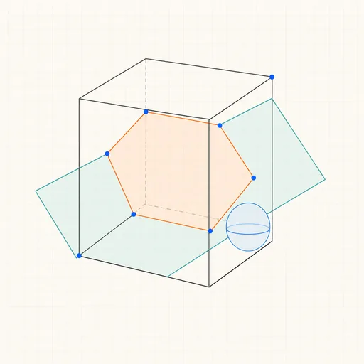
3D Geometry Board
Points, lines, planes, spheres and polyhedra on an orbiting camera — slice solids with planes, unfold nets, drop the Dandelin spheres into a cone and drag everything.
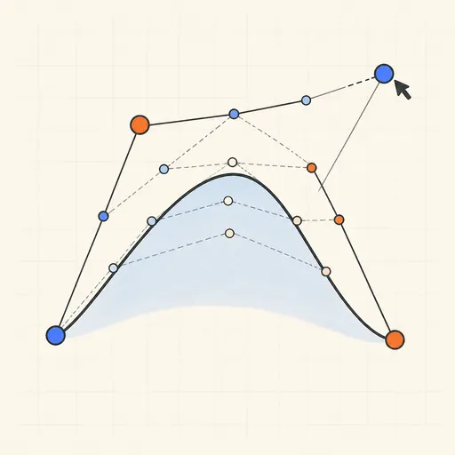
Bézier Curve Playground
Drag control points and watch De Casteljau’s algorithm construct a Bézier curve step by step.
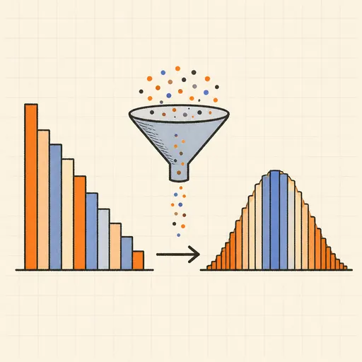
Central Limit Theorem Demo
Sample from any lopsided distribution and watch the averages pile up into a bell curve.
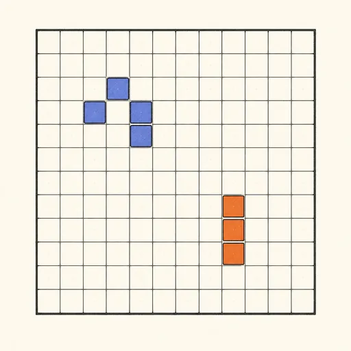
Conway’s Game of Life
Paint cells and watch Conway’s cellular automaton breed gliders, guns and oscillators.
Dynamic Geometry Board
Construct with points, lines, circles and transformations, then drag anything — the construction stays true, and a checker tells you which relations are theorems.

Fantasy Map Generator
Roll a seed and get a continent: coastlines, mountains, rivers, biomes and named towns, ready for your campaign.