Economy Sandbox, Explained

After reading this you will understand how a tiny agent-based economy turns simple household and firm rules into GDP, inflation, unemployment and inequality, and how to move the policy levers without setting off an inflation spiral.

What the sandbox is, and one thing to try first

The Economy Sandbox runs a small macroeconomy from the bottom up. It holds a few dozen households and a handful of firms. Households work, earn wages, spend part of their wealth and save the rest. Firms hire workers, produce goods, set prices by watching whether their shelves clear, and go bankrupt when they guess wrong. A government taxes income and hands the money back out. A central bank sets an interest rate or simply prints money.

No global equation says "GDP shall rise 3 percent." The macro curves you see are the sum of thousands of small local decisions. That is what makes the model interesting: it produces recessions, booms and widening wealth gaps without anyone scripting them.

Here is the first experiment worth running. Leave every lever at its default, let the economy settle for 50 steps, then double the money supply in one move. Watch the price index. Output barely changes once the workforce is already busy, but prices climb until they are roughly double. That is the quantity theory of money in miniature, and you can read it straight off the chart.

When this model helps and when it misleads

Use the sandbox to build intuition about direction and feedback: which way does unemployment move when you raise taxes, what happens to inequality when transfers stop, how a supply shock and a demand shock feel different on the same dashboard. These qualitative lessons are robust.

Do not use it to forecast a real economy. The sandbox has dozens of agents, not millions. It has one good, no trade, no banks lending to each other, no expectations about future policy. Real inflation depends heavily on what people expect inflation to be, and this model only hints at that. Treat the numbers as a teaching aid, not a prediction.

Every run uses random draws for who gets hired and who spends. Two runs with identical settings will not match exactly. Judge a policy by its average effect across several runs, not by a single trajectory.

The rules each agent follows

Households consume a fixed fraction of their current wealth each step. If a household holds wealth w_i and the marginal propensity to consume is c, its planned spending is:

S_i = c \cdot w_i

Here S_i is the spending of household i, w_i is its wealth, and c is a number between 0 and 1. With c = 0.5, a household holding 200 tries to spend 100 this step. Total demand is the sum of these across all households.

Firms adjust prices toward market clearing. If a firm sold more than it made last step, it raises its price; if it has unsold stock, it cuts. A simple version of that rule is:

p_{t+1} = p_t \cdot \left(1 + \alpha \cdot \frac{D - Q}{Q}\right)

p_t is the current price, D is quantity demanded, Q is quantity produced, and \alpha is a small adjustment speed such as 0.1. If demand exceeds supply by 20 percent, the price rises by 0.1 \times 0.2 = 0.02, that is 2 percent.

The government taxes each wage at rate \tau and redistributes the pool. With a flat transfer, each household receives the same share regardless of income, which is why taxes push the Gini coefficient down.

Measuring inequality with the Gini coefficient

The dashboard reports a Gini coefficient, a single number from 0 to 1 that summarises how uneven wealth is. A Gini of 0 means everyone holds the same amount. A Gini near 1 means one household holds almost everything. For a population of n wealth values w_i with mean \bar{w}, one convenient form is:

G = \frac{\sum_{i=1}^{n} \sum_{j=1}^{n} |w_i - w_j|}{2 n^2 \bar{w}}

The double sum adds up the absolute wealth gap between every pair of households. Dividing by 2 n^2 \bar{w} scales the result into the range 0 to 1. As one example, four households holding 10, 10, 10, 10 give G = 0, while 0, 0, 0, 40 give G = 0.75.

Inequality rises even when every household starts identical and follows the same rule. Random luck compounds: a household that earns a little more spends and saves a little more, which lets it earn more still. This multiplicative drift is why the Gini climbs on its own unless taxes or transfers pull it back.

Reproducing the money-printing demo

Run the demo with default settings. The instructive part is what happens when money supply doubles once the workforce is fully employed. Suppose the economy sits at output Q = 100 goods per step, a price index of 1.00, and a money supply M = 1000. The quantity theory writes total spending as money times how often each unit changes hands (velocity V), which equals price times output:

M \cdot V = P \cdot Q

Before the shock: 1000 \times V = 1.00 \times 100, so velocity V = 0.1.
Double the money to M = 2000. Output cannot rise because every worker is already employed, so Q stays at 100.
Velocity is a habit of spending and changes slowly, so hold V = 0.1. Then 2000 \times 0.1 = P \times 100.
Solve for the new price: P = 200 / 100 = 2.00. The price index doubles.

The sandbox will not hit exactly 2.00 because prices adjust step by step and some slack usually remains. Expect the index to climb toward roughly double over 20 to 40 steps, which the worked number brackets well.

Prices sit flat, then approach double after the money shock at step 50, matching the quantity-theory prediction of a price index near 2.00.

Reading the four gauges together

The dashboard shows GDP, inflation, unemployment and Gini at once. They only make sense as a set.

GDP: Total value of goods produced per step, price times quantity. A falling GDP with steady prices signals a demand shortfall. Rising GDP with rising prices signals an overheating boom.
Inflation: Percent change in the price index per step. A reading of 2 means prices rose 2 percent since the last step. Sustained readings above zero compound fast: 2 percent per step for 35 steps roughly doubles prices.
Unemployment: Share of households with no wage this step. It rises when firms cut output or go bust, and it is the fastest gauge to react to a demand shock.
Gini: Wealth inequality from 0 to 1, as defined above. It moves slowly and drifts up unless policy resists it.

A useful check: raise the tax rate from 0.1 to 0.3 and watch two gauges move in opposite directions. Gini falls because transfers even out wealth. GDP often dips because higher taxes trim take-home pay and therefore spending. That trade-off is the whole point of the lever.

Common mistakes when steering the economy

The first mistake is reacting to noise. A one-step jump in unemployment from 0.08 to 0.11 is often just the random draw of who got hired. Wait several steps before you conclude a trend exists.

The second mistake is overcorrecting inflation. If you slam the interest rate up the moment prices rise, you can push the economy into a recession that then needs its own rescue. Small, patient moves beat large ones.

The third mistake is confusing the two shocks. A demand shock cuts spending, so output and prices fall together. A supply shock cuts what firms can produce, so output falls while prices rise. The same fall in GDP calls for opposite responses, so read the inflation gauge before you touch a lever.

Related simulations on this site

The Economy Sandbox is an agent-based model, and several neighbours use the same bottom-up idea. Sugarscape grows a stark wealth distribution from agents foraging sugar, the closest cousin to the inequality story here. Schelling's Segregation Model shows how mild individual preferences produce sharp collective patterns, the same emergence principle.

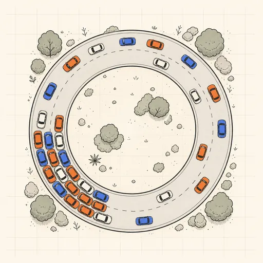
For boom-and-bust dynamics driven by feedback rather than agents, the Predator–Prey Simulator gives clean oscillations from two coupled equations. The SIR Epidemic Simulator shows a quantity rise and burn out, useful for comparing how a shock propagates. For jams that appear from nothing, see the Traffic Jam Simulator.

Frequently asked questions

Why does inflation rise even when I do not print money?

If demand outruns what firms can produce, prices climb regardless of the money supply. Firms raise prices toward market clearing, so a demand shock alone can lift inflation a few percent per step until output catches up or spending falls.

Why does inequality keep growing when all households start equal?

Spending and saving are proportional to wealth, so small random advantages compound. A household that draws a run of good luck saves more, earns more on that saving, and pulls ahead. The Gini drifts up from 0 toward higher values unless taxes and transfers push back.

Can I get zero unemployment?

Briefly, in a boom. But full employment leaves no slack, so any extra spending then goes straight into prices rather than output. Chasing zero unemployment usually trades it for higher inflation.

Why do results differ between identical runs?

Hiring and spending draw on random numbers each step. Two runs with the same levers follow different paths. Compare policies by their average across several runs, not by one trajectory.

Does doubling money always double prices?

Only once the economy is at full capacity and velocity holds steady. With idle workers, extra money first raises output, and prices rise less than proportionally. In the demo, roughly 20 percent of the money increase was absorbed by output before prices caught up.

Try it yourself in the tool