ROC Curves and Decision Thresholds, Explained
After reading this you will be able to read an ROC curve, compute TPR, FPR, precision and AUC by hand from a confusion matrix, and pick the threshold that minimizes expected cost for a given prevalence.
What a threshold actually does
A binary classifier does not output "positive" or "negative" directly. It outputs a score: a number that is meant to be larger for positives than for negatives. A logistic regression returns a probability between 0 and 1. A distance-based model returns a signed margin. In every case the final decision needs one more step: compare the score to a threshold t, call everything above it positive and everything below it negative.
That single choice controls every count in the confusion matrix. Move the threshold down and you catch more true positives, but you also flag more negatives by mistake. Move it up and you make fewer false alarms, but you miss more real positives. The score distributions do not change; only the vertical line that splits them does.
Here is the hook. Suppose negatives have scores centered at 0 and positives centered at 2, both with standard deviation 1. Put the threshold at 1.0, exactly between them. You catch about 84% of positives (TPR) and falsely flag about 16% of negatives (FPR). Slide the threshold to 1.5 and TPR drops to about 69% while FPR falls to about 7%. Same model, same data, very different behavior. The ROC curve is just the record of every such trade you could make.
The confusion matrix and the rates it produces
At any threshold, each example lands in one of four cells.
- True positive (TP)
- Actual positive, scored above the threshold. Correct alarm.
- False positive (FP)
- Actual negative, scored above the threshold. False alarm.
- False negative (FN)
- Actual positive, scored below the threshold. Missed case.
- True negative (TN)
- Actual negative, scored below the threshold. Correct pass.
Every metric on the tool is a ratio of these four counts. The two that build the ROC curve are computed within each true class:
TPR (also called recall or sensitivity) is the fraction of real positives you catch. FPR is the fraction of real negatives you wrongly flag. Specificity is 1 - \text{FPR}. Because both are normalized inside their own class, neither one changes when the class ratio changes. That property is why ROC curves are stable across prevalence, and it is also their biggest trap, covered later.
Precision mixes the classes and so does depend on prevalence:
Precision answers a different question: of everything you flagged, what fraction was right? The F_1 score is the harmonic mean of precision and recall, which pulls the result toward the smaller of the two.
Reading the ROC curve and the AUC
Plot FPR on the x-axis and TPR on the y-axis. As you sweep the threshold from very high to very low, the operating point traces a path from the bottom-left corner (0, 0), where you call nothing positive, to the top-right corner (1, 1), where you call everything positive. A perfect classifier hugs the top-left corner: TPR near 1 while FPR stays near 0. A useless classifier sits on the diagonal, where TPR equals FPR, meaning your positive calls land on real positives no more often than chance.
The area under the curve (AUC) summarizes the whole path in one number. It has a clean meaning: AUC is the probability that a randomly chosen positive scores higher than a randomly chosen negative. An AUC of 0.5 is chance. An AUC of 1.0 means the two distributions never overlap.
For two Gaussians with equal variance separated by d' (the difference in means measured in standard deviations), the AUC equals \Phi(d'/\sqrt{2}), where \Phi is the standard normal CDF. With d' = 2 this gives \Phi(1.414) \approx 0.921.
A worked example with the demo data
The demo button uses the field defaults: negatives centered at 0, positives centered at 2 (so d' = 2), both with standard deviation 1, prevalence 0.5. Work through three thresholds by hand using the standard normal CDF \Phi.
Rates at three thresholds
- At t = 1.0: TPR is the chance a positive (mean 2) exceeds 1, which is \Phi(2 - 1) = \Phi(1) \approx 0.841. FPR is the chance a negative (mean 0) exceeds 1, which is 1 - \Phi(1) \approx 0.159.
- At t = 1.5: TPR = \Phi(0.5) \approx 0.691, FPR = 1 - \Phi(1.5) \approx 0.067.
- At t = 0.5: TPR = \Phi(1.5) \approx 0.933, FPR = 1 - \Phi(0.5) \approx 0.309.
Now turn rates into counts. Take a sample of 1000 with prevalence 0.5, so 500 positives and 500 negatives. At t = 1.0: TP = 0.841 \times 500 \approx 421, FN \approx 79, FP = 0.159 \times 500 \approx 79, TN \approx 421. Precision is 421 / (421 + 79) = 0.841, equal to recall here because the classes are balanced and the setup is symmetric. Accuracy is (421 + 421)/1000 = 0.842.
| Threshold | TP | FP | TPR | FPR | Precision |
|---|---|---|---|---|---|
| 0.5 | 467 | 155 | 0.933 | 0.309 | 0.751 |
| 1.0 | 421 | 79 | 0.841 | 0.159 | 0.841 |
| 1.5 | 346 | 34 | 0.691 | 0.067 | 0.911 |
When ROC helps and when it misleads
ROC and AUC are the right summary when you care about ranking quality and want a picture that does not shift with the class ratio. They let you compare two models on the same test set independent of the base rate, and they let you pick an operating point after the fact.
They mislead when positives are rare. Because FPR divides by the large pool of negatives, a false alarm rate that looks tiny on the ROC axis can still swamp your true positives.
Suppose prevalence is 1 in 1000. At t = 1.0 you keep TPR 0.841 and FPR 0.159. In 100000 examples there are 100 positives and 99900 negatives. You catch 84 positives but raise 0.159 \times 99900 \approx 15884 false alarms. Precision collapses to 84 / (84 + 15884) \approx 0.0053. The ROC point did not move, but the classifier is now nearly useless in practice. Look at the precision-recall view whenever positives are rare.
Choosing a threshold by cost
Accuracy treats a missed cancer and a false alarm as equally bad. They rarely are. Assign a cost c_{FP} to each false positive and c_{FN} to each false negative, then pick the threshold that minimizes expected cost per example:
Here \pi is the prevalence, 1 - \text{TPR} is the miss rate and FPR is the false-alarm rate. Minimizing this leads to the likelihood-ratio rule: call an example positive when
Read the right-hand side as your evidence bar. Cheap false positives (small c_{FP}) or expensive misses (large c_{FN}) lower the bar, so you predict positive more often. Rare positives (small \pi) raise the bar. For two equal-variance Gaussians the optimal threshold sits at the score where the likelihood ratio crosses that value, which you can slide to on the tool and confirm against the marked minimum on the cost curve.
Common mistakes
Reporting AUC alone. Two models with the same AUC can behave very differently at the threshold you will actually deploy. AUC averages over all thresholds, including ones you would never use.
Comparing AUC across different test sets. AUC is stable across prevalence within one dataset, but a harder test set gives a lower AUC for the same model. Only compare on identical data.
Reading precision off the ROC curve. The ROC axes are TPR and FPR. Precision is not on the plot and depends on prevalence, as the rare-positive example showed.
Optimizing the threshold on the test set. If you sweep thresholds and pick the best one on the same data you report, you have peeked. Choose the threshold on a validation split. The Cross-Validation Visualizer shows why a single split can mislead.
Assuming a probability threshold of 0.5 is meaningful. A score of 0.5 only earns its name if the model is calibrated. Check that with the Calibration and Reliability Diagram before you trust probability cutoffs.
Related tools
Costs and prevalence turn a score into a decision, but the score itself has to mean something first. The calibration tool checks whether a predicted 0.7 really corresponds to 70% positives. To understand where a model's error comes from before you tune its threshold, see the Bias-Variance Decomposition. If your features live on wildly different scales, decisions can hinge on that alone; the Feature Scaling Demo makes the effect visible.
Frequently asked questions
What is a good AUC?
It depends on the task, but as a rough guide: 0.5 is chance, 0.7 is weak, 0.8 is useful, 0.9 and up is strong. With d' = 2 the AUC is 0.921. Do not chase a high AUC if the operating point you deploy has poor precision.
Why does my ROC curve look the same when I change prevalence?
Because TPR and FPR are computed inside each true class. Changing the ratio of positives to negatives rescales the counts but not the within-class rates. Precision and the PR curve do move, so switch to the precision-recall view to see prevalence effects.
How is AUC related to the ROC curve exactly?
It is the area under the curve, integrated from FPR 0 to 1. Equivalently it equals the probability that a random positive outscores a random negative, which you can estimate directly by counting pairs.
Should I use accuracy or F1?
Accuracy is fine when classes are balanced and costs are equal. When positives are rare, accuracy rewards a model that just predicts "negative" every time. Use precision, recall, F_1, or an explicit cost, and read them at your chosen threshold rather than averaged over all of them.
Where does the optimal threshold come from?
From the cost function above. Set the derivative to zero and you get the likelihood-ratio condition. On the tool, enter your two costs and the marked minimum on the cost curve is that optimum for the current prevalence.
Related tools
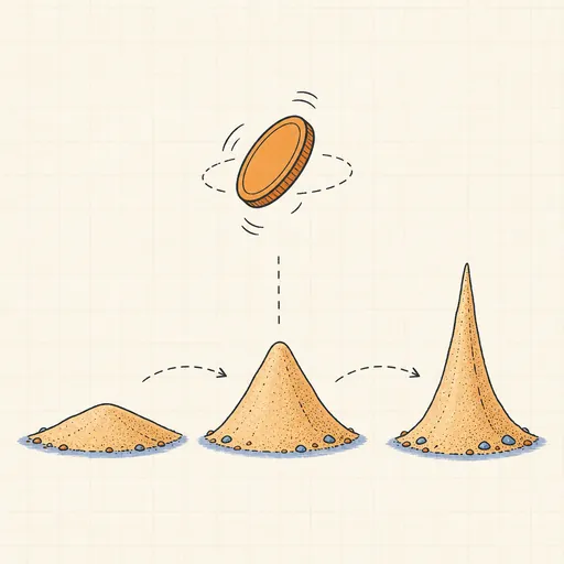
Bayesian Updating Visualizer
Flip a coin and watch a Beta prior morph into a sharpening posterior in real time.

Bias–Variance Decomposition
See bias², variance and noise split a model’s error as 50 fits wobble around the truth.
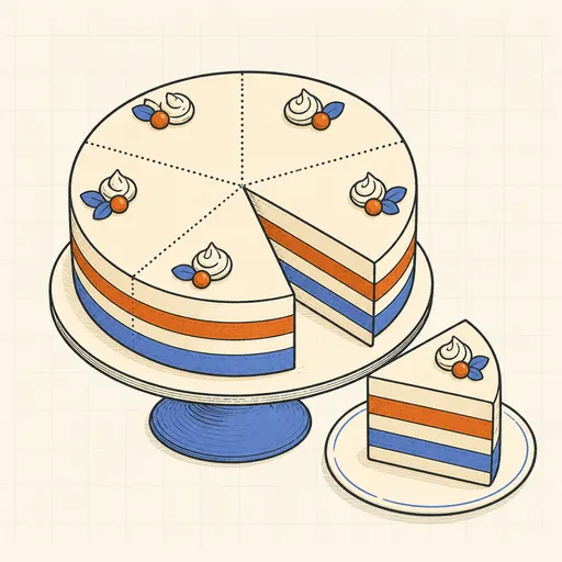
Cross-Validation Visualizer
Animate k-fold splits and see why cross-validation beats a single train/test split.
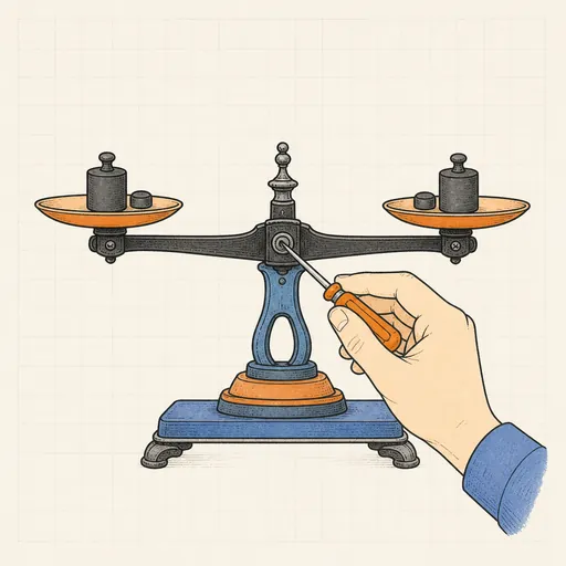
Calibration & Reliability Diagram
Check whether predicted probabilities mean what they say, then fix them with temperature scaling.
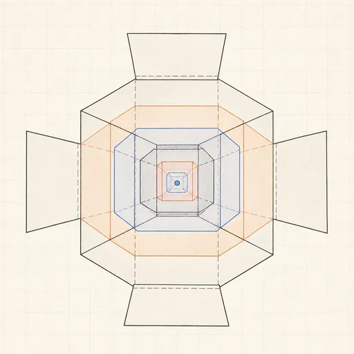
Curse of Dimensionality
Watch distances concentrate and nearest neighbors fail as dimensions pile up.
Feature Scaling Demo
Run k-means and gradient descent on raw versus scaled features and watch scaling decide the outcome.