The Perceptron, Explained
After reading this you will be able to run Rosenblatt's 1958 learning rule by hand, predict when it converges and when it cycles forever, and read the rotating decision boundary in the animation as a record of the mistakes the model has made.
What the perceptron is
A perceptron is a single artificial neuron that draws one straight line (or in higher dimensions, one flat hyperplane) and classifies every point by which side it lands on. It computes a weighted sum of the inputs, adds a bias, and reports the sign. Nothing more.
Give it two inputs x_1 and x_2. It holds a weight vector w = (w_1, w_2) and a bias b, and predicts the label as \text{sign}(w \cdot x + b). The prediction is +1 when the sum is positive and -1 when it is negative. The set of points where the sum is exactly zero is the decision boundary: a line perpendicular to w.
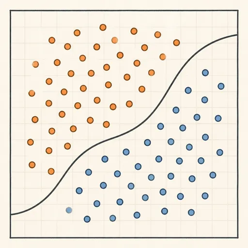
Here is the hook. Load two well-separated blobs into the animation and the boundary snaps into place after a handful of updates. Load XOR, four points arranged so no straight line can separate them, and the boundary spins forever without ever settling. That failure, published by Minsky and Papert in 1969, stalled neural network research for over a decade. The same rule that converges in six steps on easy data never stops on XOR.
When to reach for it, and when not to
The perceptron is worth your attention for what it teaches, not for what it ships. Its assumptions are strict and its output is thin.
Use it, or study it, when your two classes are linearly separable: some straight line puts every positive on one side and every negative on the other. On such data the learning rule is guaranteed to find a separating line in a finite number of steps. That guarantee is the whole point.
Do not use it when the classes overlap, because the rule never converges and just keeps flipping the boundary on whatever point it currently gets wrong. Do not use it when you need a probability rather than a hard +1 or -1; for that, reach for the Logistic Regression Playground. Do not use it when you want the widest separating gap rather than any separating line at all; the perceptron stops at the first line that works, while a support vector machine keeps going for the maximum margin (see the SVM Playground).
The update rule and why it points the right way
The perceptron learns only from mistakes. A point (x, y) with true label y \in \{-1, +1\} is misclassified when the signed score has the wrong sign:
Here w \cdot x is the dot product w_1 x_1 + w_2 x_2, and the product is at most zero exactly when the prediction disagrees with y (or lands on the line). When that happens, apply the update with learning rate \eta \gt 0:
Every symbol: w is the weight vector, x the input, y the true label, b the bias, and \eta a positive step size. Correctly classified points trigger no change at all.
Why does this help? Suppose a positive point (y = +1) got scored negative. After the update the new score on that same point is (w + \eta x) \cdot x + (b + \eta) = w \cdot x + b + \eta(\|x\|^2 + 1). The added term \eta(\|x\|^2 + 1) is strictly positive, so the score moves up, toward the correct sign. The move might not be enough to fix the point in one step, but it always pushes in the right direction. In the animation this shows as the weight arrow swinging toward the ringed point and the perpendicular boundary rotating to catch it.
Starting from w = 0 and b = 0, changing \eta only rescales every weight by the same factor. Doubling \eta doubles w and b together, which leaves every sign unchanged. So the learning rate cannot change which points get misclassified or how many updates you need. It matters only when the starting weights are nonzero.
A worked example on two blobs
Take four points, two per class, matching a small separable dataset. Use \eta = 1 and start from w = (0, 0), b = 0.
| Point | x_1 | x_2 | Label y |
|---|---|---|---|
| A | 2 | 1 | +1 |
| B | 3 | 2 | +1 |
| C | -1 | -2 | -1 |
| D | -2 | -1 | -1 |
Stepping through the updates
- Point A, score 0 \cdot 2 + 0 \cdot 1 + 0 = 0. Since y \cdot \text{score} = 0 \le 0, it is a mistake. Update: w = (0,0) + 1 \cdot 1 \cdot (2,1) = (2,1), b = 0 + 1 = 1.
- Point B, score 2 \cdot 3 + 1 \cdot 2 + 1 = 9. With y = +1, the product is 9 \gt 0. Correct, no change.
- Point C, score 2 \cdot (-1) + 1 \cdot (-2) + 1 = -3. With y = -1, the product is 3 \gt 0. Correct, no change.
- Point D, score 2 \cdot (-2) + 1 \cdot (-1) + 1 = -4. Product 4 \gt 0. Correct, no change.
- The pass over A, B, C, D produced exactly one update. Start a second pass to check for a clean sweep.
- Second pass, point A: score 2 \cdot 2 + 1 \cdot 1 + 1 = 6 \gt 0. Correct. B, C, D are unchanged from before and still correct. A full pass with zero mistakes proves convergence.
Total updates: one. Final line: 2 x_1 + x_2 + 1 = 0. The animation would ring point A once, swing the arrow to (2, 1), then run a clean pass and raise the convergence banner.
How long convergence takes
The convergence theorem gives a hard ceiling on the number of updates. If a separating line exists with margin \gamma (the smallest distance from any point to the ideal line) and all points fit inside a circle of radius R, then the number of updates is at most:
Here R is the largest \|x\| over all points and \gamma is the margin of the best possible separator. The count does not depend on how many points you have, only on this ratio. A generous gap makes the ratio small and convergence fast; a razor-thin gap makes it large.
Watch the effect. Two well-separated blobs might have R = 4 and \gamma = 2, giving a bound of (4/2)^2 = 4 updates. Push the blobs together until \gamma = 0.25 and the bound jumps to (4/0.25)^2 = 256. Same radius, sixteen times smaller margin, sixty-four times more updates allowed. In the animation this is the difference between a boundary that snaps into place and one that grinds through many passes.
Reading the animation
The status line tracks three numbers, and each one means something specific.
- Mistakes per pass
- How many points were misclassified during one sweep through the data. This is the quantity to watch. It does not fall smoothly; it can bounce up and down. Convergence is declared only when it hits zero.
- Total updates
- The running count of weight changes. Compare it against (R/\gamma)^2 to see how much slack the bound gives.
- Epochs
- Complete passes over the dataset. One clean epoch with zero mistakes ends training.
The weight arrow starts at the origin and grows as updates accumulate. Its direction is the normal to the boundary: the boundary line is always perpendicular to the arrow. When a point gets ringed and the update fires, the arrow tilts toward that point (for a positive) or away from it (for a negative), and the boundary rotates in step. A convergence banner appears the moment a full pass rings nobody.
If the mistake count keeps oscillating and never reaches zero, that is not a bug. It is the signature of non-separable data. The rule is doing exactly what it must: chasing a line that does not exist.
Common mistakes and misreadings
Expecting the loss to fall monotonically. The perceptron does not minimize a smooth loss like Linear Regression Playground does. It reacts to individual mistakes, so the mistake count can rise after an update that fixes one point but breaks another. Only the final zero matters.
Blaming the learning rate for slow convergence. From zero weights, \eta cannot change the number of updates. If it feels slow, the cause is a small margin, not the step size. Check (R/\gamma)^2 instead.
Thinking the found line is the best line. The perceptron stops at the first separator with zero mistakes, and that line can sit awkwardly close to one class. It does not maximize the margin. If you need robustness to new points near the boundary, the maximum-margin line from an SVM is a different objective.
Waiting for XOR to converge. It will not, ever. XOR needs a curved or piecewise boundary, which a single neuron cannot draw. The fix is hidden layers, the subject of later neural network models.
Related tools on this site
The perceptron sits at the root of a family. Follow these to see what changing the objective or the model does.
For a probability output instead of a hard sign, and a genuine smooth loss minimized by gradient descent, see the Logistic Regression Playground. For the maximum-margin version of the same separating-line idea, with kernels for curved boundaries, use the SVM Playground. For a completely different, non-parametric take on classification, the k-Nearest Neighbors Explorer votes among close points. To see boundaries built from axis-aligned splits rather than one line, grow a Decision Tree Builder, then watch many trees vote in Random Forest Voting or stack on residuals in Gradient Boosting Step-by-Step. For a probabilistic classifier with strong independence assumptions, try the Naive Bayes Classifier Demo, and to see how model complexity trades against generalization, open the Overfitting Sandbox.
Frequently asked questions
Does the perceptron always find a solution?
Only on linearly separable data. There the convergence theorem guarantees it stops after at most (R/\gamma)^2 updates. On overlapping or XOR-style data it cycles indefinitely and never declares convergence.
Why does XOR break it?
XOR labels the corners (0,0) and (1,1) one way and (0,1) and (1,0) the other. No single straight line can separate those two groups. A perceptron only draws one line, so it fails by construction. Hidden layers add more lines that combine into a nonlinear boundary.
What does the learning rate actually change?
Starting from zero weights, nothing about which points are misclassified or how many updates run: it just scales w and b uniformly, leaving every sign the same. It changes the trajectory only when you start from a nonzero weight vector, where the relative size of the step versus the existing weights matters.
How is the perceptron different from logistic regression?
Both draw a linear boundary, but the perceptron outputs a hard +1 or -1 and updates only on mistakes, while logistic regression outputs a probability between 0 and 1 and minimizes a smooth cross-entropy loss by gradient descent. Logistic regression handles overlapping classes gracefully; the perceptron does not converge on them.
What are margin and radius in the convergence bound?
The radius R is the largest distance from the origin to any data point, so R = \max \|x\|. The margin \gamma is the smallest distance from any point to the best possible separating line. Tight-margin data has small \gamma, which makes (R/\gamma)^2 large and convergence slow.
Related tools
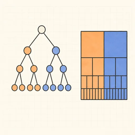
Decision Tree Builder
Grow a CART decision tree split by split and watch the partition map and tree diagram build together.
Function Sketch Finder
Sketch a curve on a zoomable coordinate grid and search dozens of function families for the equations that fit it best.
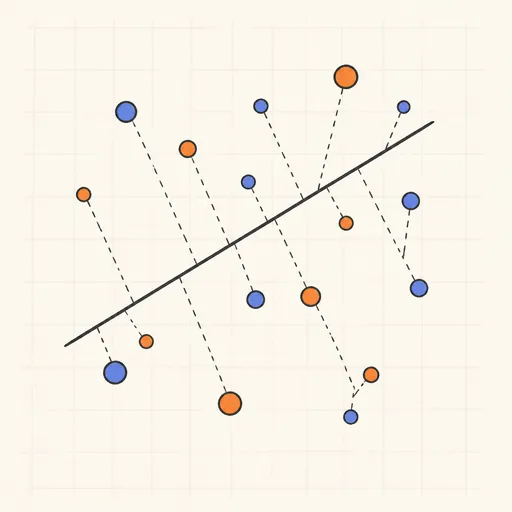
Linear Regression Playground
Place points, watch the least-squares line follow, and see gradient descent crawl across the loss surface.
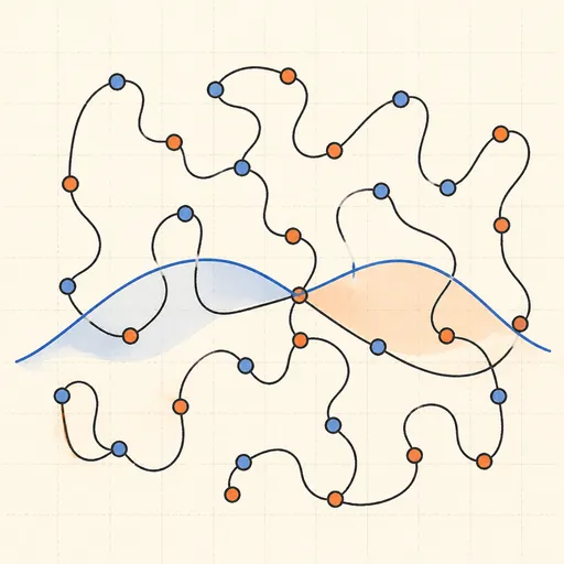
Overfitting Sandbox
Crank a polynomial’s degree on noisy data and watch the train/test error curves split apart.
Logistic Regression Playground
Paint two classes of points and watch logistic regression carve out its probability boundary by gradient descent.

Naive Bayes Classifier Demo
Score your own message with a word-count spam filter, or watch Gaussian naive Bayes classify 2D points.