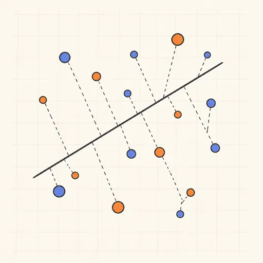
Linear Regression Playground
Ordinary least squares fits the line minimising the sum of squared vertical distances to the data, and here you build the data yourself: click empty space to add a point, drag one to move it, click one to delete it — the fitted line, slope, intercept, R² and mean squared error update instantly. Toggle the residual segments to see exactly what is being minimised, and load presets showing a clean linear trend, the pull a single outlier exerts on the fit, and a curved dataset a straight line underfits. A second canvas draws the loss surface over (slope, intercept) as contours with the closed-form solution marked — press Play and gradient descent walks the surface toward the same point the formula reaches in one step.
Runs 100% in your browser — models are trained and computed locally on your device.
Read the full guide to this tool
Notes
- Closed form: slope = Σ(x−x̄)(y−ȳ) / Σ(x−x̄)² and intercept = ȳ − slope·x̄, the unique minimum of the MSE, which is a convex paraboloid in the two parameters.
- Squared error grows quadratically with distance, so a single far-off outlier can drag the whole line — the reason robust alternatives such as least absolute deviations exist.
- R² compares the model’s squared error with that of a horizontal line at ȳ: 1 is a perfect fit, 0 means no better than predicting the mean for everything.
- With uncentred x values the loss surface is a stretched valley: gradient descent zigzags quickly down the steep slope direction but crawls along the flat intercept direction.
- Runs 100% in your browser — models are trained and computed locally on your device.
Related tools
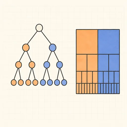
Decision Tree Builder
Grow a CART decision tree split by split and watch the partition map and tree diagram build together.
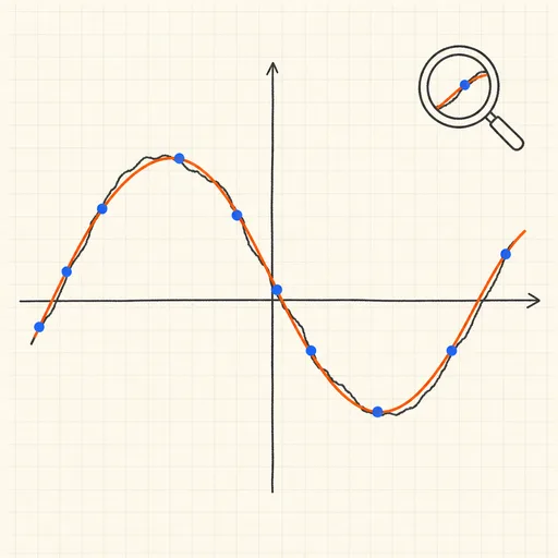
Function Sketch Finder
Sketch a curve on a zoomable coordinate grid and search dozens of function families for the equations that fit it best.

Overfitting Sandbox
Crank a polynomial’s degree on noisy data and watch the train/test error curves split apart.
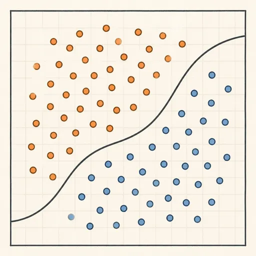
Logistic Regression Playground
Paint two classes of points and watch logistic regression carve out its probability boundary by gradient descent.

Naive Bayes Classifier Demo
Score your own message with a word-count spam filter, or watch Gaussian naive Bayes classify 2D points.
Perceptron Learning Animation
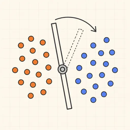
Step through Rosenblatt’s 1958 learning rule and watch the decision boundary rotate with every mistake.