Linear Regression, Explained
After reading this you will be able to compute a least-squares line by hand, read its slope, intercept, R² and mean squared error, and explain why gradient descent walks to the same answer the closed-form formula reaches in one step.
What linear regression does
Linear regression fits a straight line to a cloud of points. The line predicts an output y from an input x. You choose the line by one rule: make the sum of squared vertical gaps between the points and the line as small as possible.
Here is the hook. Take three points: (1, 2), (2, 2), (3, 5). The mean of x is 2, the mean of y is 3. The best line through them has slope 1.5 and intercept 0. It does not pass through any of the three points exactly. It passes where the total squared miss is smallest. Move any point in the playground and the line jumps to the new minimum instantly, because the answer is a formula, not a search.
The vertical gaps have a name: residuals. A residual is the actual y minus the predicted y. Squaring each residual and adding them up gives the quantity being minimised. Toggle the residual segments in the tool to see exactly those gaps.
When to use it, and when not to
Use linear regression when you believe the relationship between x and y is roughly a straight line, and you want a model you can read off in two numbers. Slope tells you how much y changes per unit of x. Intercept tells you the predicted y when x is zero. Both are interpretable, which is why the method survives despite being over 200 years old.
Avoid it, or extend it, in three situations. First, when the trend curves: a straight line cannot bend, so it underfits. The curved-data preset in the tool shows this directly. Second, when a few points sit far from the rest: squared error punishes distance quadratically, so outliers pull hard. Third, when the output is a category rather than a number. For a yes/no output, reach for the Logistic Regression Playground instead.
Linear regression assumes the noise around the line is roughly symmetric and similar in size across the range of x. When the spread fans out or the errors are heavily skewed, the fitted line is still the least-squares answer, but its interpretation as a good predictor weakens.
The formula and why it looks like that
The model predicts \hat{y} = a x + b, with slope a and intercept b. The loss to minimise is the mean squared error over n points:
Here x_i and y_i are the coordinates of point i, and n is the number of points. This function is a bowl (a convex paraboloid) in the two parameters, so it has exactly one lowest point. Setting both partial derivatives to zero and solving gives the closed form:
The numerator sums how x and y move together around their means \bar{x} and \bar{y}. The denominator sums how much x spreads around its mean. Slope is covariation divided by variation. The intercept then pins the line so it passes through the point of averages:
That single fact, that the least-squares line always passes through (\bar{x}, \bar{y}), is worth remembering. It means the line balances the points like a seesaw around their centre of mass.
A worked example you can reproduce
Load the clean-trend sample and use the three points (1, 2), (2, 2), (3, 5). Every number below can be checked with a calculator.
Fitting the line to three points
- Means: \bar{x} = (1 + 2 + 3)/3 = 2, \bar{y} = (2 + 2 + 5)/3 = 3.
- Centred products:
(1−2)(2−3) = 1,(2−2)(2−3) = 0,(3−2)(5−3) = 2. Numerator sum =3. - Centred squares of
x:(1−2)² = 1,(2−2)² = 0,(3−2)² = 1. Denominator sum =2. - Slope: a = 3 / 2 = 1.5.
- Intercept: b = 3 - 1.5 \times 2 = 0.
The fitted line is \hat{y} = 1.5 x. Now check the fit. Predictions are 1.5, 3, 4.5. Residuals are 2−1.5 = 0.5, 2−3 = −1, 5−4.5 = 0.5. Squared residuals are 0.25, 1, 0.25, summing to 1.5. Mean squared error is 1.5 / 3 = 0.5.
Reading R-squared and mean squared error
Mean squared error is in squared y units, so its size depends on your data scale. It answers "how far off, on average, squared?" but it does not tell you whether the fit is good in relative terms. That is what R^2 is for. It compares your model's squared error against the squared error of the dumbest reasonable model: a flat line at \bar{y}.
The numerator is the model's residual sum of squares. The denominator is the total sum of squares, the error you get by predicting the mean for everything. For the worked example, the residual sum is 1.5. The total sum is (2−3)² + (2−3)² + (5−3)² = 1 + 1 + 4 = 6. So R^2 = 1 - 1.5/6 = 0.75.
Read that as: the line explains 75% of the variation in y that a flat mean line left unexplained. A value of 1 means the line passes through every point. A value of 0 means the line does no better than the mean. Negative values are possible if you force a bad line onto the data, but ordinary least squares on the same data never produces a negative R^2.
How gradient descent reaches the same point
The closed form gives the answer in one step, so why animate gradient descent at all? Because most models have no closed form, and the walk across the loss surface is how they are actually trained. Linear regression is the cleanest place to watch the walk, since you can mark the exact target the formula reaches.
Gradient descent starts at some (a, b) and repeatedly steps downhill on the MSE bowl. The gradient (the direction of steepest increase) has two parts:
Each step subtracts a fraction of the gradient, set by the learning rate \eta: new a = old a minus \eta times its gradient, and likewise for b. Because the surface is a single bowl, the walk always ends at the same minimum, no matter where it starts.
If the descent zigzags and crawls, your x values are probably large and uncentred, which stretches the bowl into a long narrow valley. Centring x by subtracting its mean makes the valley round, so descent heads almost straight to the minimum. This is why real pipelines standardise features before training.
Common mistakes
Four traps catch people repeatedly.
- Trusting a high R² blindly
- A straight line through a strongly curved dataset can still post a respectable R². Look at the residual pattern. If residuals bend in a systematic arc rather than scattering, the line is underfitting.
- Letting one outlier steer the fit
- The outlier preset shows a single point dragging the slope. Squared error is the cause. If your data has genuine outliers, consider least absolute deviations, which minimises the sum of unsquared distances and reacts far less to one extreme point.
- Extrapolating past the data
- The line is only evidence within the range of
xyou observed. Predicting atxfar outside that range assumes the straight-line relationship continues, which the data never checked. - Reading slope as cause
- A slope of 1.5 means
ytends to rise by 1.5 whenxrises by 1 in this sample. It is not proof that changingxwould changey. Correlation in the fit does not establish causation.
Where to go next
Linear regression is the root of a large family. For classifying points rather than predicting a number, the Logistic Regression Playground replaces the line with an S-curve and trains by the same gradient-descent idea. To see the oldest learning rule that rotates a boundary on every mistake, try the Perceptron Learning Animation. For boundaries drawn by margins and support vectors, the SVM Playground is the next step. If you want to see a curved regression built from many small trees rather than one line, the Gradient Boosting Step-by-Step demo stacks residual fits. And to watch what happens when a model chases noise, the Overfitting Sandbox splits train and test error apart as you crank a polynomial degree.
Frequently asked questions
Why squared errors and not absolute errors?
Squaring makes the loss smooth and gives a clean closed-form solution, since the derivative is linear in the parameters. Absolute error has no single tidy formula and resists outliers more, so it is the go-to robust alternative when a few extreme points would otherwise dominate.
Can R² be negative?
Not for ordinary least squares fitted on the same data, because the fitted line can never do worse than the mean it is compared against. Negative values appear only when you evaluate a line on data it was not fitted to, or force a fixed line onto the numbers.
Does gradient descent find a different answer than the formula?
No. The MSE surface is a single convex bowl, so both reach the same minimum. In the example that is slope 1.5, intercept 0. Gradient descent only takes many small steps to arrive where the formula lands in one.
What learning rate should gradient descent use?
Small enough that each step reduces the loss, large enough to reach the minimum in a reasonable number of steps. If the loss oscillates or blows up, the rate is too high. If it barely moves, the rate is too low, or the x values need centring to reshape the valley.
How many points do I need?
Two points define a line exactly with zero error, which tells you nothing about noise. You need enough points that the trend is visible above the scatter. Even five or six make R² and MSE meaningful, as the worked example and the outlier widget show.
Related tools

Decision Tree Builder
Grow a CART decision tree split by split and watch the partition map and tree diagram build together.
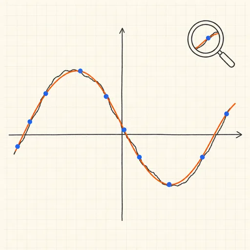
Function Sketch Finder
Sketch a curve on a zoomable coordinate grid and search dozens of function families for the equations that fit it best.
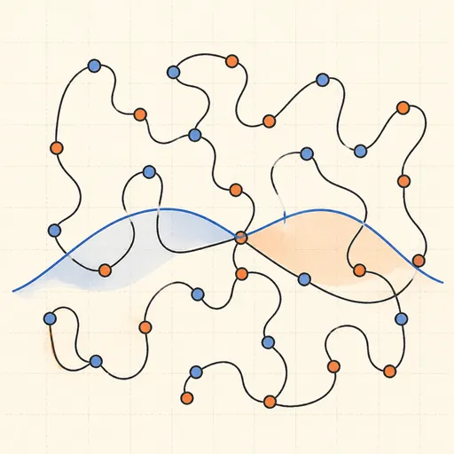
Overfitting Sandbox
Crank a polynomial’s degree on noisy data and watch the train/test error curves split apart.
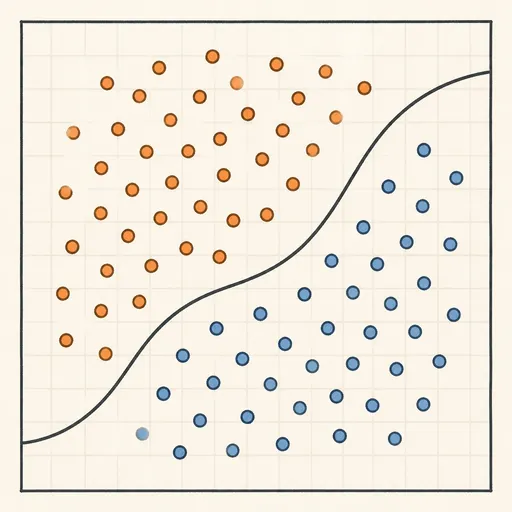
Logistic Regression Playground
Paint two classes of points and watch logistic regression carve out its probability boundary by gradient descent.

Naive Bayes Classifier Demo
Score your own message with a word-count spam filter, or watch Gaussian naive Bayes classify 2D points.
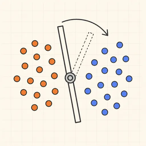
Perceptron Learning Animation
Step through Rosenblatt’s 1958 learning rule and watch the decision boundary rotate with every mistake.