Naive Bayes, Explained
After reading this you will be able to hand-compute a naive Bayes spam score, read each word's contribution as a log-likelihood ratio, and explain exactly why the model draws axis-aligned ellipses and where that assumption breaks.
What naive Bayes does, with one worked hook
Naive Bayes assigns a label to an input by asking a single question: given the features, which class is more probable? It answers with Bayes' rule, then makes one simplifying assumption to keep the arithmetic cheap.
Here is the hook. Suppose the word free appears three times as often in spam as in legitimate mail (ham), and the word meeting appears four times as often in ham. A message with both words gets two votes that pull in opposite directions. Naive Bayes adds those votes on a log scale, folds in a prior belief about how common spam is, and reports the class with the larger total. That is the whole model. The rest of this article shows the exact numbers.
The word "naive" names the assumption: features are treated as independent once the class is fixed. That is almost never true in real text. The words free and offer travel together in spam. Naive Bayes pretends they do not. The surprise is that this wrong assumption still classifies well, because the model only needs the larger score to land on the right class, not to report calibrated probabilities.
When to reach for it, and when not
Naive Bayes fits problems with many weakly informative features and limited training data. Text classification is the classic case: thousands of possible words, each a small clue. Training is one pass of counting, so it scales to large vocabularies without iterative optimization.
Skip it when features are strongly correlated and you need trustworthy probability estimates, or when a decision boundary that bends with the data matters. Because each Gaussian class is modeled with one variance per axis, the boundaries it can draw are limited. If your classes overlap along a tilted diagonal, the model cannot capture that tilt.
Use naive Bayes as a fast, honest baseline. It trains in one pass and gives you a number to beat before you spend time on logistic regression, an SVM, or a tree ensemble.
The formula and why each piece is there
Bayes' rule turns the quantity you want, the probability of a class given the features, into quantities you can estimate by counting.
Here P(c) is the prior probability of class c (how common spam is before you read the message), P(x_i \mid c) is the probability of feature x_i under that class, and the denominator is the same for every class, so it cancels when you compare classes. The product over features is the naive independence assumption written down: the joint likelihood is treated as the product of per-feature likelihoods.
Multiplying many small probabilities underflows to zero, so the demo works in logs. Comparing spam to ham reduces to one sum of differences.
Each bracketed term is one word's log-likelihood ratio. If the total is positive, spam wins. This is why each bar in the demo stacks: evidence adds. The first term on the right is the prior's contribution, present even before any word is read.
Word probabilities come from counts, but a raw count of zero would multiply the whole class to zero. Laplace smoothing fixes that.
Here \text{count}(w, c) is how often word w appeared in class c, N_c is the total word count in that class, V is the vocabulary size, and \alpha is the smoothing strength. Setting \alpha = 1 pretends you saw every vocabulary word one extra time in each class.
A worked spam example you can reproduce
Scoring "free money now"
Take a tiny vocabulary of size V = 4 with these training counts, a spam prior of 0.5, and \alpha = 1. Spam has N_{\text{spam}} = 20 total words; ham has N_{\text{ham}} = 20.
| Word | Spam count | Ham count |
|---|---|---|
| free | 9 | 1 |
| money | 6 | 2 |
| now | 3 | 3 |
| meeting | 2 | 14 |
- Smoothed probabilities use denominator N_c + \alpha V = 20 + 4 = 24. For spam:
freeis (9+1)/24 = 0.4167,moneyis (6+1)/24 = 0.2917,nowis (3+1)/24 = 0.1667. - For ham:
freeis (1+1)/24 = 0.0833,moneyis (2+1)/24 = 0.125,nowis (3+1)/24 = 0.1667. - Log-likelihood ratio for
free: \ln(0.4167) - \ln(0.0833) = -0.875 - (-2.485) = 1.609. Strong spam vote. - For
money: \ln(0.2917) - \ln(0.125) = -1.232 - (-2.079) = 0.847. Spam vote. - For
now: \ln(0.1667) - \ln(0.1667) = 0. This word is neutral; it says nothing about the class. - Prior term with equal priors: \ln(0.5/0.5) = 0. Sum the votes: 1.609 + 0.847 + 0 + 0 = 2.456.
The total log-odds is +2.456, so spam wins. Convert to a probability: 1/(1 + e^{-2.456}) = 0.921. The model reports about a 92 percent chance of spam.
now and the equal prior contribute nothing. The bars sum to the final log-odds of 2.456.Reading the results without fooling yourself
Three things in the output repay close reading. First, the sign and height of each bar. A tall positive bar means the word is far more common in spam than ham; the height is a log ratio, not a probability. Second, words outside the vocabulary are skipped entirely. They cannot vote, so a message of all-unknown words falls back to the prior alone. Third, the reported probability is often overconfident.
That overconfidence is the direct cost of the independence assumption. If free and offer almost always co-occur, the model counts them as two independent clues when they are really close to one. It multiplies their evidence twice, so probabilities get pushed toward 0 or 1. This is why the earlier footnote matters: naive Bayes only needs the argmax right. A predicted 0.999 and a true 0.85 land on the same label.
Do not read the reported percentage as a calibrated probability. Because correlated words double-count evidence, naive Bayes routinely outputs values like 0.999 when the honest figure is closer to 0.9. Trust the class it picks, not the exact number.
Gaussian mode and the tilt it cannot see
For continuous 2D points, the per-word probabilities are replaced by a Gaussian density on each axis. Each class gets a mean and a variance per feature, fit by the usual sample formulas.
Here \mu_{c,j} and \sigma_{c,j}^2 are the mean and variance of feature j in class c. The independence assumption again multiplies the two per-axis densities. Because there is no covariance term between x_1 and x_2, every class contour is an ellipse whose axes align with the coordinate axes. It cannot tilt.
Load the correlated preset in the tool to see the failure. When the true data runs along a 45-degree diagonal, the fitted ellipse still stands upright. The model wastes probability mass on empty corners and starves the diagonal where the points actually live. The classification can still work if the classes are far apart, but the fitted shape visibly misses the structure.
Try the assumption yourself
Common mistakes
- Setting alpha to zero
- With no smoothing, a single word never seen in one class drives that class probability to zero, and no other evidence can recover it. Keep \alpha \ge 1 unless you have a specific reason not to.
- Trusting the probability
- The reported confidence is inflated by correlated features. Treat it as a ranking, not a calibrated risk.
- Feeding correlated features to Gaussian mode
- Height and weight, or two lags of the same signal, violate independence badly. The upright ellipse cannot represent the tilt, so the fit suffers.
- Ignoring the prior
- If spam is only 5 percent of your mail, a 50 percent prior overpredicts spam. Set the prior to the real base rate. A prior of
0.05subtracts \ln(0.05/0.95) = -2.944 from every log-odds before any word is read.
Where to go next
Naive Bayes is one baseline among several. To compare its straight-line-ish boundary with a probabilistic model that fits a boundary by optimization, try the Logistic Regression Playground. For a boundary that bends and a margin you can watch, the SVM Playground is the natural next step. If you want to see a model memorize the training data and then fail on new points, the Overfitting Sandbox makes the train and test error split apart. For a distance-based alternative that also votes, see the k-Nearest Neighbors Explorer, and for a rule-based partition, the Decision Tree Builder.
Frequently asked questions
Why is it called "naive"?
Because it assumes every feature is independent of the others once the class is known. In text that is false: words like free and offer co-occur. The name flags the assumption honestly. The method works anyway when you only need the top class.
What does Laplace smoothing actually change?
It adds \alpha to every count and \alpha V to every total, so an unseen word gets a small nonzero probability instead of zero. With \alpha = 1, a word seen 0 times in a class of 20 words and vocabulary 4 gets 1/24 = 0.0417 rather than 0.
Why does the demo add logs instead of multiplying probabilities?
Multiplying hundreds of numbers below 1 underflows to zero in floating point. Taking logs turns the product into a sum, which is numerically stable and lets each word appear as one additive bar.
Can naive Bayes handle more than two classes?
Yes. Compute the score for each class and pick the largest. The two-class log-odds shortcut is just a convenience; with three or more classes you compare full log-scores directly.
Why do the Gaussian ellipses never tilt?
The model fits one variance per feature and no covariance between features. A tilted ellipse requires an off-diagonal covariance term, which the independence assumption sets to zero. So the contours always align with the axes.
Related tools
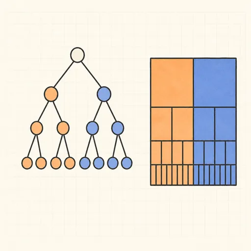
Decision Tree Builder
Grow a CART decision tree split by split and watch the partition map and tree diagram build together.
Function Sketch Finder
Sketch a curve on a zoomable coordinate grid and search dozens of function families for the equations that fit it best.
Linear Regression Playground
Place points, watch the least-squares line follow, and see gradient descent crawl across the loss surface.
Overfitting Sandbox
Crank a polynomial’s degree on noisy data and watch the train/test error curves split apart.
Logistic Regression Playground
Paint two classes of points and watch logistic regression carve out its probability boundary by gradient descent.
Perceptron Learning Animation
Step through Rosenblatt’s 1958 learning rule and watch the decision boundary rotate with every mistake.