Logistic Regression, Explained
After reading this you will be able to write down the logistic regression model and its cross-entropy loss, derive the gradient descent update by hand, reproduce the numbers the playground shows, and read its probability heatmap without fooling yourself.
What logistic regression does
Logistic regression predicts the probability that a point belongs to one class. In the playground you paint blue points (call them class 0) and orange points (class 1), and the model learns a function that returns a number between 0 and 1 for every location on the plane. The heatmap shades that number: deep blue near 0, deep orange near 1, pale in between. The pale band where the probability equals exactly 0.5 is the decision boundary.
Here is the hook. Load the two separable blobs and press Play. Within a few dozen epochs the boundary snaps between the clouds and accuracy hits 1.0. Now load the circle nested inside a ring. The straight boundary cannot separate a disc from the annulus around it, so accuracy stalls near 0.5. Toggle degree-2 polynomial features and press Play again: the boundary bends into an ellipse and accuracy climbs. Same algorithm, different feature space.
When to use it, and when not
Reach for logistic regression when you want calibrated probabilities and an interpretable model, and when a linear boundary (in whatever features you supply) is roughly right. It trains fast, rarely overfits with a little regularization, and every weight has a plain meaning: it is the change in the log-odds per unit of that feature.
Do not expect it to carve curved boundaries on its own. With raw x and y it can only draw a straight line. The circle dataset proves this. You have two escapes: add features by hand (the degree-2 toggle) or switch to a model that builds nonlinearity for you, such as the Decision Tree Builder or the k-Nearest Neighbors Explorer.
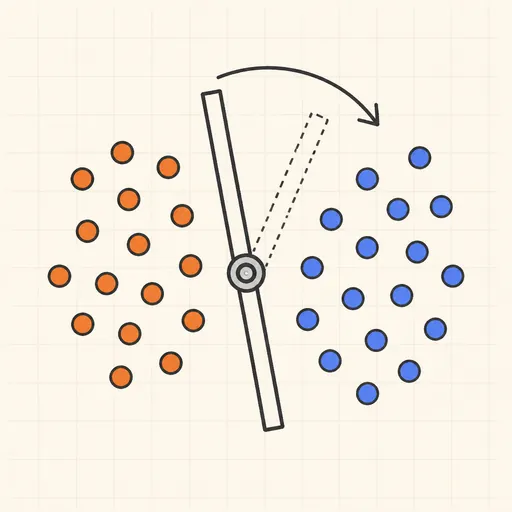
Logistic regression and the Perceptron Learning Animation both draw a linear boundary, but they train differently. The perceptron nudges its weights only on misclassified points and stops once every point is correct. Logistic regression always minimizes a smooth loss and reports a probability, so it keeps refining confidence even after accuracy reaches 1.0.
The model and its loss
The model computes a linear score, then squashes it through the sigmoid.
Here \mathbf{x} is the input point, \mathbf{w} is the weight vector, b is the bias, and z is the raw score. The sigmoid maps any real z into (0, 1). At z = 0 it returns exactly 0.5, which is why the decision boundary is the line \mathbf{w} \cdot \mathbf{x} + b = 0.
To train, you need a loss that punishes confident wrong answers. That is the cross-entropy (log loss) for one example with true label y \in \{0, 1\} and predicted probability p = \sigma(z):
When y = 1 the loss is -\ln p, which is 0 when p = 1 and grows without bound as p \to 0. When y = 0 it is -\ln(1 - p), the mirror image. A prediction of 0.9 on a true 1 costs -\ln 0.9 \approx 0.105; a prediction of 0.1 on that same point costs -\ln 0.1 \approx 2.303. Confident and wrong is expensive.
The gradient, and why it is so clean
Gradient descent needs the derivative of the average loss with respect to each weight. The sigmoid and the log loss were chosen to fit together, and the algebra collapses to something memorable:
The term (\sigma(z_i) - y_i) is the prediction error for point i: predicted probability minus true label. Multiply it by the input and average over all n points. This is the exact form used by the Linear Regression Playground, where the error is (\hat{y}_i - y_i). The only change is that here the prediction passes through a sigmoid first.
Each epoch takes one step downhill:
The learning rate \eta is the step size set by the slider. Too small and the boundary crawls; too large and the loss can bounce or diverge.
One epoch by hand on four points
Use a tiny separable set: two blue points at (-2, 0) and (-1, 1) with y = 0, two orange points at (2, 0) and (1, -1) with y = 1. Start from w_1 = 0, w_2 = 0, b = 0, so every score is 0 and every prediction is \sigma(0) = 0.5. Use \eta = 1.
- Errors (p_i - y_i) at the start: point 1 gives
0.5 - 0 = 0.5, point 2 gives0.5, point 3 gives0.5 - 1 = -0.5, point 4 gives-0.5. - Gradient for w_1: average of e_i \cdot x_i = \tfrac{1}{4}(0.5 \cdot -2 + 0.5 \cdot -1 + -0.5 \cdot 2 + -0.5 \cdot 1) = \tfrac{1}{4}(-1 - 0.5 - 1 - 0.5) = -0.75.
- Gradient for w_2: \tfrac{1}{4}(0.5 \cdot 0 + 0.5 \cdot 1 + -0.5 \cdot 0 + -0.5 \cdot -1) = \tfrac{1}{4}(0 + 0.5 + 0 + 0.5) = 0.25.
- Gradient for b: average of the errors = \tfrac{1}{4}(0.5 + 0.5 - 0.5 - 0.5) = 0.
- Update with \eta = 1: w_1 = 0 - (-0.75) = 0.75, w_2 = 0 - 0.25 = -0.25, b = 0.
Check the orange point (2, 0) after this one step: z = 0.75 \cdot 2 - 0.25 \cdot 0 + 0 = 1.5, so p = \sigma(1.5) \approx 0.818. It moved from 0.5 toward its true label of 1. The symmetric blue point (-2, 0) now scores z = -1.5, p \approx 0.182. One epoch already split the classes.
Watching the loss and the weights grow
Keep running that separable example and the loss keeps dropping, but it never reaches 0 and the weights never stop growing. On perfectly separable data the model can always lower the loss a little more by scaling \mathbf{w} up, pushing every prediction closer to a hard 0 or 1. The boundary stops moving, yet the numbers behind it inflate forever. The chart below shows log loss falling toward zero while the weight norm climbs without limit.
Nudge the L2 slider off zero to stop the runaway. L2 adds a penalty \lambda \lVert \mathbf{w} \rVert^2 to the loss, whose gradient 2\lambda \mathbf{w} pulls weights back toward zero every step. This caps the weight norm, keeps probabilities from saturating at exactly 0 and 1, and makes the model's confidence more honest.
Try the effect of L2 yourself
The single idea worth playing with is how regularization strength trades off fit against confidence. Move the slider and watch both the weight size and the sharpness of the boundary respond.
Reading the heatmap without fooling yourself
Three things on the screen carry the meaning. The 0.5 line is the boundary: the set of points where \mathbf{w} \cdot \mathbf{x} + b = 0. It is straight with raw features and a conic section (ellipse, parabola or hyperbola) with degree-2 features. The color strength is confidence, not correctness: a deep orange region only means the model assigns high probability there, which can still be wrong. The accuracy counts how many training points land on the correct side of 0.5.
Watch for the gap between loss and accuracy. On overlapping clouds accuracy might plateau at 0.85 while the loss keeps drifting down, because the model is still adjusting probabilities on points it already classifies correctly. High accuracy with low confidence (pale colors everywhere) usually means strong L2 or few epochs. Perfect accuracy with blinding colors on separable data is the runaway weights from the previous section.
Common mistakes
Do not read a deep-color region as proof the model is right there. On the overlapping-clouds preset the model will paint a point solid orange and still be wrong 15% of the time in that zone. Confidence is the model's estimate, not a guarantee, and unregularized fits systematically overstate it.
A few more traps. First, a learning rate that is too high makes the loss curve jump around or shoot up instead of down; halve \eta and try again. Second, expecting a straight line to solve the circle: no amount of training helps, because the boundary family is wrong until you add polynomial features. Third, reading raw weight magnitudes as importance when features are on different scales, since a weight absorbs the units of its feature. Fourth, confusing this with the perceptron or a hard SVM: those optimize different objectives and give no probability. If margins interest you, the SVM Playground shows the maximum-margin view of the same 2D data.
What toy demos can and cannot tell you
This playground trains a full-batch model on a handful of hand-painted points in two dimensions. That is enough to see the update rule, the boundary, and the effect of regularization with your own eyes. It is not enough to draw conclusions about production systems, which run on thousands of features, use mini-batch or stochastic updates, add early stopping and validation splits, and worry about class imbalance and calibration on held-out data. Treat the demo as a microscope on the mechanism, not a benchmark. To see how flexible models pay for extra capacity with variance, the Overfitting Sandbox makes the train/test split visible.
Frequently asked questions
Why use cross-entropy instead of squared error for classification?
Squared error paired with a sigmoid gives a non-convex loss with flat regions where gradients nearly vanish, so training stalls. Cross-entropy is convex in the weights and its gradient stays proportional to the error (p - y), so a confidently wrong point still produces a strong correction. That is why a wrong prediction of 0.01 against a true 1 costs -\ln 0.01 \approx 4.6 and pushes hard, while squared error would cost only 0.99^2 \approx 0.98.
How do polynomial features let a linear model draw a circle?
Adding x^2, xy and y^2 means the score becomes w_1 x + w_2 y + w_3 x^2 + w_4 xy + w_5 y^2 + b. Setting that to zero is the general equation of a conic. The model is still linear in its weights, so the same gradient works, but the boundary in the original (x, y) plane can now be an ellipse that wraps the inner disc.
What does the bias term do?
The bias b shifts the boundary without rotating it. In the worked example the bias gradient was 0 because the errors were symmetric, so the line stayed centered. Give the classes unequal counts or an off-center split and b moves to compensate, the same way an intercept shifts a regression line.
Why does accuracy jump in steps while loss falls smoothly?
Loss is a continuous function of the weights, so it changes a little every epoch. Accuracy counts points on the correct side of 0.5, which only changes when a point actually crosses the boundary. Between crossings accuracy is flat even as the loss keeps dropping.
Can I get probabilities I can trust from this?
On clean, well-regularized data the probabilities are reasonable, but the demo does no calibration and no held-out check. An unregularized fit on separable data reports near-certain probabilities that are an artifact of unbounded weights, not real evidence. Add L2 and judge confidence against a separate test set before believing any single number.
Related tools
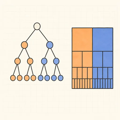
Decision Tree Builder
Grow a CART decision tree split by split and watch the partition map and tree diagram build together.
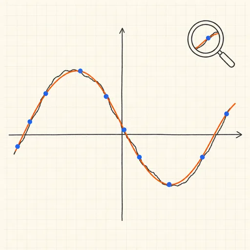
Function Sketch Finder
Sketch a curve on a zoomable coordinate grid and search dozens of function families for the equations that fit it best.
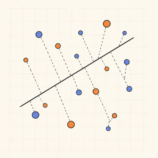
Linear Regression Playground
Place points, watch the least-squares line follow, and see gradient descent crawl across the loss surface.
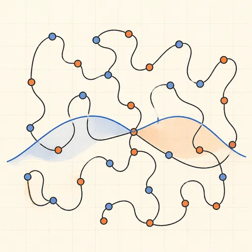
Overfitting Sandbox
Crank a polynomial’s degree on noisy data and watch the train/test error curves split apart.

Naive Bayes Classifier Demo
Score your own message with a word-count spam filter, or watch Gaussian naive Bayes classify 2D points.
Perceptron Learning Animation
Step through Rosenblatt’s 1958 learning rule and watch the decision boundary rotate with every mistake.