k-Nearest Neighbors, Explained
After reading this you can classify a point by hand with k-nearest neighbors, pick a sensible k using leave-one-out accuracy, and recognize the bias-variance trade-off in the shape of a decision map.
What k-nearest neighbors does
k-nearest neighbors (kNN) is the simplest classifier that still works. To label a new point, you find the k training points closest to it, let them vote, and assign the majority class. There is no training step. The data is the model.
Here is the hook. Suppose you have red points clustered on the left of a map and blue points clustered on the right. Drop a new point at (3, 4). Its three nearest labels turn out to be red, red, blue. The vote is 2 to 1, so the point is red. Move it one step right and the vote can flip to blue. Every location on the map gets a color this way, and those colors tile into regions: the decision map you see in the Explorer.
Because there is no fitting, all the work happens at prediction time. You store the points, then measure distances on demand. That makes kNN easy to reason about and slow to query on large data, a trade-off worth understanding before you reach for it.
When to use it, and when not
kNN shines when the decision boundary is irregular and you have no reason to assume a particular shape. A straight-line model like the Logistic Regression Playground assumes the boundary is linear. kNN assumes nothing about global shape; it only trusts local neighborhoods. If similar inputs really do share labels, kNN captures that directly.
It struggles in three situations. First, high dimensions: in many dimensions almost all points sit at nearly the same distance, so "nearest" stops meaning much. Second, large datasets: a single query scans every stored point, so with 1,000,000 points every prediction costs 1,000,000 distance computations. Third, features on different scales: a feature measured in thousands will dominate a feature measured in tenths unless you standardize first.
Always scale your features before running kNN. If one axis ranges 0 to 1000 and another ranges 0 to 1, the first axis contributes about 1000^2 = 1{,}000{,}000 to squared distance while the second contributes at most 1. The small feature is invisible. Standardize each column to mean 0 and standard deviation 1 first.
The distance formula and the vote
Everything rests on a distance. For two points p = (p_1, p_2) and q = (q_1, q_2), Euclidean distance is the straight line:
The symbols p_1, q_1 are the x-coordinates and p_2, q_2 the y-coordinates. Manhattan distance instead sums the absolute coordinate gaps:
The two differ in shape. All points at Euclidean distance 1 form a circle; all points at Manhattan distance 1 form a diamond. That is why switching to Manhattan in the Explorer makes the boundaries turn axis-aligned.
Once you have distances, the plain vote counts each of the k neighbors equally. Distance-weighted voting gives each neighbor weight 1/d, so a neighbor at distance 0.5 counts 2.0 while a neighbor at distance 4 counts 0.25. The predicted class is the one with the largest total weight:
Here N_k is the set of the k nearest neighbors, d_i is the distance to neighbor i, y_i is its class, and the bracket is 1 when the neighbor belongs to class c and 0 otherwise.
A worked example you can reproduce
Classifying one point by hand
Take six training points across two classes and one query point at q = (4, 4).
| Point | x | y | Class | Distance to (4,4) |
|---|---|---|---|---|
| A | 3 | 4 | Red | 1.000 |
| B | 5 | 5 | Red | 1.414 |
| C | 6 | 3 | Blue | 2.236 |
| D | 4 | 2 | Blue | 2.000 |
| E | 1 | 1 | Blue | 4.243 |
| F | 7 | 7 | Red | 4.243 |
- Sort by distance: A (1.000, Red), B (1.414, Red), D (2.000, Blue), C (2.236, Blue), then E and F tied at 4.243.
- For
k = 3the neighbors are A, B, D. Votes: Red 2, Blue 1. Prediction is Red. - For
k = 5add C and E. Votes: Red 2, Blue 3. Prediction flips to Blue. - Now try distance-weighted voting at
k = 5. Red weight is 1/1.000 + 1/1.414 = 1.707. Blue weight is 1/2.000 + 1/2.236 + 1/4.243 = 1.183. Prediction returns to Red.
One point, three different answers, depending on k and weighting. That sensitivity is the whole lesson. The close red pair dominates once you count distance, but a plain count at k = 5 lets three scattered blue points outnumber them.
Choosing k with leave-one-out accuracy
You cannot judge k by how well the model labels its own training data. At k = 1 every training point is its own nearest neighbor, so accuracy is a perfect 100% and tells you nothing. Leave-one-out cross-validation fixes this: to score point i, remove it, classify it with the remaining points, and check whether the label matches. Repeat for all points and average.
Here n is the number of training points and \hat{y}_i^{(-i)} is the prediction for point i when point i is held out. The bracket is 1 for a correct prediction. The Explorer sweeps this across every k from 1 to 25 and charts it.
The curve usually rises, peaks, then falls. Small k overfits: the boundary chases every noisy point, so leave-one-out accuracy is mediocre because held-out points often sit next to noise. Large k underfits: the neighborhood spans multiple classes and washes out real structure. The peak is your sweet spot.
Reading the decision map
The colored background is the prediction for every location. At k = 1 the map is the Voronoi diagram of your points: each region is exactly the set of locations closer to one training point than to any other. Boundaries are jagged and every training point is classified correctly, which is the textbook picture of overfitting.
Raise k and the islands merge into smoother regions. A single mislabeled point that owned a whole island at k = 1 gets outvoted by its neighbors at k = 7 and disappears from the map. Push k too high and thin true regions vanish too, which is underfitting.
Prefer odd k for two-class problems so a simple majority vote cannot tie. With three classes a tie is still possible (for example 2-2-1 at k=5 is fine, but 1-1-1 at k=3 is a three-way tie), so distance weighting is a useful tiebreaker: it almost never produces an exact tie because real distances rarely match.
Common mistakes
- Skipping feature scaling
- Unscaled features let the widest-range column dominate the distance. Standardize first, every time.
- Reading training accuracy as skill
- At
k = 1training accuracy is always 100%. Use leave-one-out or a held-out test set instead. - Picking k blindly
- A common rule of thumb is k \approx \sqrt{n}, so for
n = 100you might start neark = 10. Treat it as a starting point, not an answer; the leave-one-out curve is the real guide. - Even k in two-class problems
- An even
kinvites ties that get broken arbitrarily. Use oddkor distance weighting. - Ignoring query cost
- Each prediction scans all stored points. kNN reads as free because there is no training, but every query pays the full price.
Related tools on this site
kNN draws no explicit boundary; other classifiers do. The SVM Playground finds a maximum-margin boundary and, with kernels, curved ones. The Perceptron Learning Animation shows the oldest learning rule rotating a line with each mistake. For rule-based partitions rather than distance-based ones, grow a Decision Tree Builder, then watch many trees smooth a jagged boundary in Random Forest Voting. To see the same bias-variance story with a polynomial degree instead of k, open the Overfitting Sandbox. For probability-based classification compare the Naive Bayes Classifier Demo. If you want regression rather than classification, start with the Linear Regression Playground, and for staged trees see Gradient Boosting Step-by-Step.
Frequently asked questions
What is the best value of k?
There is no universal answer. Sweep k with leave-one-out accuracy and take the peak. On the three-blob data charted above the peak sits near k = 9 at about 0.95. A rough starting guess is k \approx \sqrt{n}.
Does kNN have a training phase?
No. It stores the points and does all computation at query time. That is why it is called a lazy or instance-based method. The cost moves from training to prediction.
Why does the boundary become smoother as k grows?
A larger neighborhood averages over more points, so a single odd point cannot control the vote. At k = 1 one mislabeled point owns a whole Voronoi cell; at k = 7 its six neighbors outvote it and the cell disappears.
Euclidean or Manhattan distance?
Euclidean is the default and matches straight-line intuition. Manhattan can help when features are independent axes measured in different units, and it produces axis-aligned, diamond-shaped neighborhoods. Try both and compare leave-one-out accuracy.
How accurate can kNN get?
Cover and Hart proved in 1967 that as the dataset grows, the error of 1-NN is at most twice the Bayes-optimal error, the best any classifier could achieve. Larger k can bring you closer to that optimum on clean, low-dimensional data.
Related tools
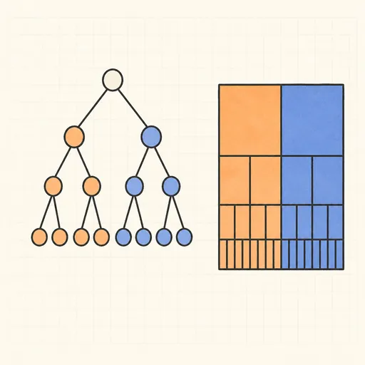
Decision Tree Builder
Grow a CART decision tree split by split and watch the partition map and tree diagram build together.
Function Sketch Finder
Sketch a curve on a zoomable coordinate grid and search dozens of function families for the equations that fit it best.
Linear Regression Playground
Place points, watch the least-squares line follow, and see gradient descent crawl across the loss surface.
Overfitting Sandbox
Crank a polynomial’s degree on noisy data and watch the train/test error curves split apart.
Logistic Regression Playground
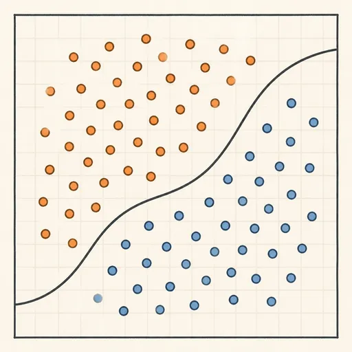
Paint two classes of points and watch logistic regression carve out its probability boundary by gradient descent.
Naive Bayes Classifier Demo
Score your own message with a word-count spam filter, or watch Gaussian naive Bayes classify 2D points.