Decision Trees, Explained
After reading this you will know how a CART tree picks each split, how Gini and entropy measure impurity, how to read the partition map and tree diagram together, and why axis-aligned cuts struggle with a slanted boundary.
What a decision tree does
A decision tree splits the feature space into rectangular regions, one cut at a time, and assigns every region a single predicted class. Each internal node asks one yes-or-no question of the form x_j \le t: is feature j at most the threshold t? Points that pass go left, the rest go right. You repeat this on each side until a stopping rule fires. The leaves hold the final predictions.
Here is the hook. Load the checkerboard preset in the builder. A straight line cannot separate those four alternating blocks, so a linear model does poorly. A tree, though, can carve the plane into a grid of boxes. With enough depth it isolates each block and reaches high accuracy. The tree does not learn one global rule. It learns a stack of local ones.
Because every cut is a single threshold on a single feature, the boundaries are always parallel to an axis. That fact drives both the strengths and the weaknesses you will see below.
When to use one, and when not
A single decision tree is worth reaching for when you want a model you can read off as a flowchart, when your features are on different scales and you do not want to standardize them, and when the true class boundaries are roughly box-shaped. Trees handle mixed numeric ranges without preprocessing because each split only compares one feature to one threshold.
Skip a lone tree when the boundary is smooth and slanted, when you need a calibrated probability rather than a hard region, or when you want the last few points of accuracy. A single tree is high variance: move a handful of training points and the whole structure can change. That instability is exactly why ensembles exist. The Random Forest Voting tool averages many randomized trees, and Gradient Boosting Step-by-Step stacks shallow trees on residuals. Both trade the readable flowchart for a steadier boundary.
A tree with no depth limit will keep splitting until every leaf is pure. On clean data that reaches 100% training accuracy, which sounds good but usually means the tree has fit noise. The stopping rules exist to prevent this.
The impurity formula and why it works
CART chooses each split greedily: it tries every feature and every candidate threshold, and it keeps the one that most reduces impurity. Impurity measures how mixed the class labels are inside a node. A node that is all one class has impurity zero.
The tool offers two impurity measures. The Gini index for a node is
where p_k is the fraction of samples in the node that belong to class k. Entropy is the alternative:
Both peak when classes are evenly mixed and drop to zero when one class dominates. For a two-class node that is half and half, Gini is 1 - (0.5^2 + 0.5^2) = 0.5 and entropy is -(0.5\log_2 0.5 + 0.5\log_2 0.5) = 1 bit.
A split sends the node's samples into a left child and a right child. The quality of the split is the impurity decrease, weighting each child by its share of the samples:
Here n is the parent sample count, n_L and n_R are the counts in the left and right children, and I_L and I_R are their impurities. CART evaluates \Delta I for every possible split and takes the largest.
A worked split you can check by hand
First split on a two-class node
Take a node with 20 samples: 12 of class A and 8 of class B. Suppose a candidate threshold sends 10 samples left (9 A, 1 B) and 10 samples right (3 A, 7 B). Work the Gini impurity decrease.
- Parent shares: p_A = 12/20 = 0.6, p_B = 0.4. Parent Gini = 1 - (0.6^2 + 0.4^2) = 1 - (0.36 + 0.16) = 0.48.
- Left child: p_A = 0.9, p_B = 0.1. Gini = 1 - (0.81 + 0.01) = 0.18.
- Right child: p_A = 0.3, p_B = 0.7. Gini = 1 - (0.09 + 0.49) = 0.42.
- Weighted child impurity: (10/20)(0.18) + (10/20)(0.42) = 0.09 + 0.21 = 0.30.
- Impurity decrease: 0.48 - 0.30 = 0.18.
Now test a worse threshold: 10 left (6 A, 4 B) and 10 right (6 A, 4 B). Each child has Gini 1 - (0.36 + 0.16) = 0.48, the weighted impurity is still 0.48, and the decrease is 0.48 - 0.48 = 0. That split tells you nothing, so CART rejects it in favor of the first one, which scored 0.18.
Reading the partition map and the tree diagram
The builder draws two views of the same model. The partition map shades every region by its majority class, so you see the boxes the tree has carved. The tree diagram below grows a node for each split, labelled with its sample count and impurity. Match them up: the root node's cut is the first line drawn on the map, and each deeper node refines one of the existing regions.
Read a leaf this way. A leaf labelled "n=14, Gini=0.13, class A" contains 14 training samples, is nearly pure, and predicts A. A leaf with "Gini=0.5" is a coin flip between two classes and contributes little. Watch the impurity numbers fall as you descend: that is the tree buying certainty with each split.
The accuracy readouts use a fixed 70/30 train/test split. Training accuracy tells you how well the tree fits the data it grew on. Test accuracy, computed on the held-out 30%, estimates how it will do on new points. When those two numbers diverge, the gap is your overfitting.
The axis-aligned weakness
Load the diagonal preset. The true boundary is a single slanted line: class A below it, class B above. A linear model draws that line with one weight vector. A tree cannot. Every cut it makes is vertical or horizontal, so it approximates the diagonal with a staircase.
To see why this costs so much, picture a diagonal running corner to corner. One horizontal cut plus one vertical cut make an L-shaped step that misclassifies the triangle in the corner. To halve the error you double the steps, and to halve it again you double them once more. The number of cuts needed grows without bound as you demand a finer approximation, while a straight line would need exactly one parameter.
If your boundary looks slanted or curved, try a model built for it before adding tree depth. The Logistic Regression Playground and the SVM Playground both draw oblique boundaries directly, and SVM kernels handle curves.
Common mistakes
The first mistake is reading a deep tree as truth. A tree grown to depth 12 on 100 points can hit 100% training accuracy while its test accuracy sits far lower. That gap is memorized noise, not learned structure. Set the maximum depth and the minimum samples per leaf deliberately, then watch the test number rather than the train number.
The second is trusting a single tree's exact splits. Because CART is greedy and high variance, swapping a few points can flip which feature the root uses. Do not over-interpret one threshold as a discovered law. If you need stable structure, average many trees.
The third is expecting probabilities. A leaf's class share (say 11 of 14 are class A) is a rough estimate, but it comes from a small sample and jumps in coarse steps. Treat tree outputs as regions, not as well-calibrated probabilities.
Do not compare training accuracy across depths and conclude that deeper is better. Training accuracy almost always rises with depth. The honest comparison is test accuracy, and it usually peaks at a modest depth and then falls.
Related tools
Once a single tree makes sense, see how it fits the wider family. The k-Nearest Neighbors Explorer also builds jagged, non-linear boundaries but from distance rather than splits, which is a useful contrast. The Perceptron Learning Animation and Linear Regression Playground show the linear methods a tree is not. The Naive Bayes Classifier Demo offers a probabilistic alternative for the same two-dimensional problems. To feel overfitting in isolation, without trees at all, crank the polynomial degree in the Overfitting Sandbox and watch the train and test curves split apart.
Frequently asked questions
Should I use Gini or entropy?
They almost always produce similar trees. Gini is slightly cheaper because it avoids a logarithm, and it tends to isolate the most frequent class into its own branch. Entropy sometimes prefers more balanced splits. On the presets here the resulting boundaries are usually identical or very close, so pick either and focus on depth.
Why does my tree keep splitting until every leaf is pure?
Because that is CART's default behavior with no limits. A node stops only when it is pure, when it hits the maximum depth, or when splitting would leave a leaf below the minimum sample count. Raise the minimum samples per leaf or lower the maximum depth to stop earlier.
Do I need to scale my features first?
No. Each split compares one feature to one threshold, so multiplying a feature by 10 just multiplies its thresholds by 10. The tree structure is unchanged. This is a genuine convenience compared with distance-based or gradient-based methods.
Why is a random forest better than one tree?
A single tree is high variance: its splits swing with small changes in the data. Averaging many trees, each grown on a bootstrap sample with random feature subsets, cancels much of that variance. The result is a smoother boundary and higher test accuracy, at the cost of the readable flowchart.
Can a tree handle more than two classes?
Yes. The impurity formulas sum over all classes, so three-class data works the same way. The builder lets you place points of three classes, and each leaf simply predicts whichever class is the majority of the samples that reach it.
Related tools
Function Sketch Finder
Sketch a curve on a zoomable coordinate grid and search dozens of function families for the equations that fit it best.
Linear Regression Playground
Place points, watch the least-squares line follow, and see gradient descent crawl across the loss surface.
Overfitting Sandbox
Crank a polynomial’s degree on noisy data and watch the train/test error curves split apart.
Logistic Regression Playground
Paint two classes of points and watch logistic regression carve out its probability boundary by gradient descent.

Naive Bayes Classifier Demo
Score your own message with a word-count spam filter, or watch Gaussian naive Bayes classify 2D points.
Perceptron Learning Animation
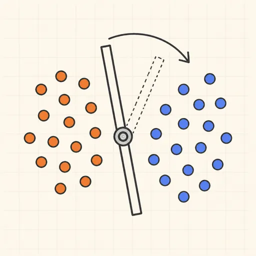
Step through Rosenblatt’s 1958 learning rule and watch the decision boundary rotate with every mistake.