Cross-Validation, Explained
After reading this you will know how k-fold cross-validation estimates a model's error on unseen data, how to compute the estimate by hand, and why a single train/test split can lie to you.
What cross-validation is
You fit a model to answer one question: how will it behave on data it has not seen? The training error will not tell you, because a flexible model can memorize its training set and score near zero there while failing on anything new. You need to score the model on points it never touched during fitting.
The simplest way is a holdout split: train on 70% of the data, test on the remaining 30%. That works, but the number you get depends on which points happened to land in the test set. Cross-validation removes that luck. It cuts the data into k equal parts called folds, holds out each fold once as a test set, trains on the other k-1 folds, and averages the k test errors.
Here is the hook. Take 30 noisy points from a sine curve and fit a degree-9 polynomial. A single 70/30 split might report a validation mean squared error (MSE) of 0.18 on one shuffle and 0.61 on the next. Same model, same data, different luck. Five-fold cross-validation on the same 30 points gives a stabler number with a standard deviation you can read directly, so you can tell whether degree 9 truly beats degree 3 or just got a friendly split.
When to use it, and when not
Use cross-validation when data is limited and every point is expensive to collect, because it reuses each point for both training and testing. Use it to compare models or tune a hyperparameter (here, the polynomial degree) when a single holdout would be too noisy to separate the candidates.
Do not use plain k-fold when the rows are not independent. Time series need forward-chaining splits so the future never leaks into the past. Grouped data (many rows per patient, per user, per image) needs group-aware folds so the same group does not sit in both training and test. And do not cross-validate a step you already ran on the full data: if you selected features or scaled columns using all rows before splitting, the folds are contaminated and the estimate is too optimistic.
Any preprocessing that learns from data (scaling, feature selection, target encoding, PCA) must be fit inside each fold using only that fold's training rows. Fit it once on everything and your reported error is a fantasy.
The formula and the intuition
Split the n rows into k folds F_1, \ldots, F_k of roughly equal size. For each fold i, train a model \hat{f}_{-i} on all rows except F_i, then score it on F_i. The cross-validation estimate is the average of the fold errors.
Reading the symbols: |F_i| is the number of points in fold i, y_j is the true target for point j, and \hat{f}_{-i}(x_j) is the prediction from the model that never saw fold i. The inner average is the MSE on one fold; the outer average combines the k folds. Every point is predicted exactly once, by a model that did not train on it.
The intuition: instead of trusting one holdout, you build k holdouts that together cover the whole dataset, then average. Averaging k estimates cuts the variance of the estimate. Leave-one-out is the extreme k = n: each fold is a single point, so you fit n models. It is almost unbiased, but the n models are nearly identical (they differ by one row), so their errors are highly correlated and the average can still be noisy. That is why k = 5 or k = 10 is the usual compromise.
A worked example on the demo data
The demo fits a polynomial to noisy points from y = \sin(2\pi x). To keep the arithmetic checkable, work through 5-fold cross-validation with 10 points and a degree-3 fit. Suppose the five folds produce these MSE values after each refit.
| Fold | Held-out points | Validation MSE |
|---|---|---|
| 1 | 2 | 0.042 |
| 2 | 2 | 0.118 |
| 3 | 2 | 0.067 |
| 4 | 2 | 0.201 |
| 5 | 2 | 0.089 |
Computing the mean and spread by hand
- Sum the fold MSEs:
0.042 + 0.118 + 0.067 + 0.201 + 0.089 = 0.517. - Divide by k = 5: the CV estimate is
0.517 / 5 = 0.1034. - Find deviations from the mean:
-0.0614, 0.0146, -0.0364, 0.0976, -0.0144. - Square and sum them:
0.003770 + 0.000213 + 0.001325 + 0.009526 + 0.000207 = 0.015041. - Divide by k and take the root for the population standard deviation: \sqrt{0.015041 / 5} = \sqrt{0.003008} \approx 0.0548.
Report it as 0.103 \pm 0.055. Fold 4 at 0.201 is nearly five times fold 1 at 0.042, which is why a single holdout landing on fold 4 alone would have badly overstated the error. The average tames that.
Reading the results the tool shows
The tool gives you two numbers and a picture. The mean estimates the error you expect on new data. The standard deviation tells you how much that estimate would wobble if you shuffled and refolded. A mean of 0.10 with spread 0.05 is a different situation than 0.10 with spread 0.01: in the first case you cannot confidently claim a rival model at 0.08 is better, because the folds disagree by more than that gap.
Next to those numbers the tool draws a histogram of 30 separate 70/30 splits. Watch how wide it is. It is common for those 30 single-split errors to range from 0.05 to 0.35 for the same model on the same data. The whole point of the histogram is to make the luck-of-the-split variance visible: one holdout draws one bar from that distribution, and you would never know how far from the center you landed.
The CV estimate is nearly unbiased for a model trained on (k-1)/k of the data. With k = 5 that is 80% of the rows, so the estimate slightly over-states the error of your final model, which you train on 100%. This pessimism is small and shrinks as k grows.
An interactive to feel the split variance
Move k and the sample size and watch two things at once: the width of the single-split histogram, and the standard deviation of the k-fold estimate. The lesson lands when you see the histogram stay wide while the CV band tightens.
Common mistakes
The mistakes below each produce a number that looks fine and is wrong.
- Leaking preprocessing across folds
- Scaling or feature selection fit on all rows before splitting lets test rows influence training. The estimate drops below the true error, sometimes far below.
- Not shuffling ordered data
- If the rows are sorted by the target or by time, unshuffled folds are not representative. Shuffle before splitting for independent rows; do not shuffle time series.
- Choosing the model on the same CV you report
- If you try 12 degrees and report the best CV score, that score is optimistic because you selected on noise. Use nested cross-validation, or hold out a final untouched test set.
- Reading the mean and ignoring the spread
- A mean of
0.103with spread0.055does not justify picking it over a model at0.090. The fold disagreement is larger than the gap. - Comparing MSE across different sample sizes
- Larger training sets usually lower error. Compare models at a fixed n and fixed k, not across different settings.
Related tools
Cross-validation estimates error but does not tell you what kind of error you have. The Bias–Variance Decomposition splits a model's error into bias², variance and noise, which explains why a degree-9 fit on 30 points has high variance in the first place. If your task is classification rather than regression, the ROC & Threshold Explorer shows how the decision threshold trades false positives against false negatives, and the Calibration & Reliability Diagram checks whether predicted probabilities match observed frequencies. When preprocessing matters, the Feature Scaling Demo shows why scaling belongs inside the fold. For a wider view of why high-dimensional data breaks distance-based methods, see the Curse of Dimensionality, and for the idea of an estimate sharpening as evidence accumulates, the Bayesian Updating Visualizer.
Frequently asked questions
How many folds should I use?
Five or ten for most problems. Both give a good balance between bias (each model trains on 80% or 90% of the data) and the compute cost of fitting that many models. Use leave-one-out only when data is very scarce, and expect its estimate to be noisier despite lower bias.
Is cross-validation better than a single train/test split?
For estimating error on limited data, yes, because it averages away the luck of one split and reports a standard deviation. A single large holdout is fine when data is plentiful and refitting many times is expensive. The tool's histogram of 30 splits shows exactly how much one split can vary.
Which model do I actually deploy after cross-validation?
Refit on all the data using the degree or hyperparameters that cross-validation preferred. The k models fit during cross-validation exist only to estimate error; you discard them. The final model trained on 100% of the data will usually be slightly better than the CV number, because CV trained on only (k-1)/k of it.
Why does my CV score change every time I run it?
Because shuffling before splitting uses a random order, and the fold assignment changes. Fix the random seed for reproducibility, and report the standard deviation so a small change between runs is expected rather than alarming.
Does cross-validation prevent overfitting?
No. It measures overfitting; it does not fix it. If a degree-12 polynomial on 30 points has high variance, cross-validation reports a high error and a large spread, which tells you to pick a simpler model. The fix is choosing a less flexible model or adding regularization, not the estimate itself.
Related tools
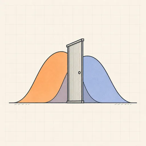
ROC & Threshold Explorer
Drag a decision threshold and watch the confusion matrix, ROC curve and expected cost respond in real time.
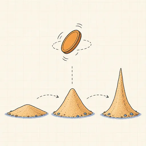
Bayesian Updating Visualizer
Flip a coin and watch a Beta prior morph into a sharpening posterior in real time.

Bias–Variance Decomposition
See bias², variance and noise split a model’s error as 50 fits wobble around the truth.
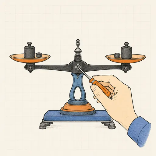
Calibration & Reliability Diagram
Check whether predicted probabilities mean what they say, then fix them with temperature scaling.
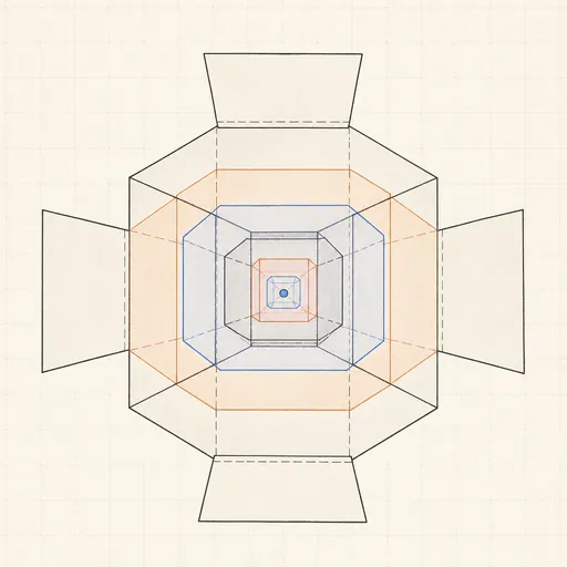
Curse of Dimensionality
Watch distances concentrate and nearest neighbors fail as dimensions pile up.
Feature Scaling Demo
Run k-means and gradient descent on raw versus scaled features and watch scaling decide the outcome.