Bias-Variance Decomposition, Explained
After reading this you will be able to split any regression model's expected error into three named parts, compute each part by hand on a small example, and read the tradeoff off a complexity sweep instead of guessing.
What the decomposition says
Train a model, and its error on new data comes from three sources that do not overlap. First, the model class may be too rigid to match the truth, so even its best average fit misses. That gap is bias. Second, each training set is a random draw, so the fit wobbles from one sample to the next. That scatter is variance. Third, the targets themselves carry noise you cannot predict from the inputs. That floor is irreducible noise.
Here is the hook. Fit a degree-1 line to a sine curve on 50 different training sets. Every line lands in nearly the same place (low variance), but they all sit far from the wiggling truth (high bias). Now fit a degree-12 polynomial to the same 50 sets. The average curve tracks the sine almost perfectly (bias near zero), but the individual fits fly apart, some shooting to +8 where the truth is 0 (huge variance). Neither extreme wins. The best total error sits somewhere in between, and this tool shows you exactly where.
When the split is exact, and when it is not
The clean three-way split holds for squared-error loss on a regression target. Under squared loss the cross terms cancel algebraically, so the total is a plain sum with no leftover. That is why the tool uses squared loss and draws a stacked bar: the three heights literally add up to the expected error.
The decomposition is a thinking tool, not a production diagnostic you can measure directly. To compute variance you need many independent training sets from the same distribution. In real work you get one training set, so you estimate the tradeoff indirectly through resampling and held-out data.
For classification with 0-1 loss the neat "bias² + variance + noise" identity does not hold: the terms interact and can even reduce error together. Use this decomposition for regression under squared loss, and reason about it qualitatively elsewhere.
The formula and what each symbol means
Fix an input x. Let f(x) be the true function and let the observed target be y = f(x) + \varepsilon with noise variance \sigma^2. Let \hat{f}_D(x) be the model fitted on training set D. Averaging over both the random D and the random noise gives:
The first term is bias squared, where \bar{f}(x) = E[\hat{f}_D(x)] is the average fit across all training sets. The second term is variance, the average squared distance of each fit from that average. The third term \sigma^2 is the noise variance, which no model can remove because it lives in the targets, not the fit.
Read the roles cleanly. Bias measures how far the center of your fits sits from the truth. Variance measures how spread out the fits are around their own center. Noise is fixed by the data-generating process.
A worked example you can check by hand
Use the demo defaults: true function sine, evaluate at the probe point x = 0.5, where f(0.5) = \sin(2\pi \cdot 0.5) = 0. Suppose you fit five training sets (the tool uses 50, but five is enough to see the arithmetic) and each returns a prediction at x = 0.5. Let the noise variance be \sigma^2 = 0.04.
Bias² and variance at x = 0.5
Five fits predict these values at the probe:
| Fit | Prediction | Deviation from mean | Squared deviation |
|---|---|---|---|
| 1 | 0.30 | 0.06 | 0.0036 |
| 2 | 0.10 | -0.14 | 0.0196 |
| 3 | 0.40 | 0.16 | 0.0256 |
| 4 | 0.20 | -0.04 | 0.0016 |
| 5 | 0.20 | -0.04 | 0.0016 |
- Average fit: \bar{f}(0.5) = (0.30 + 0.10 + 0.40 + 0.20 + 0.20)/5 = 0.24.
- Bias: f(0.5) - \bar{f}(0.5) = 0 - 0.24 = -0.24. Bias squared is (-0.24)^2 = 0.0576.
- Variance: average of the squared deviations, (0.0036 + 0.0196 + 0.0256 + 0.0016 + 0.0016)/5 = 0.052/5 = 0.0104.
- Noise: \sigma^2 = 0.04, given.
- Expected error: 0.0576 + 0.0104 + 0.04 = 0.108.
So at this probe the model's error is dominated by bias (0.0576), with variance (0.0104) and noise (0.04) smaller. That is the signature of a model that is still slightly too rigid at x = 0.5. Add flexibility and the 0.0576 shrinks while the 0.0104 grows.
Watching the tradeoff move
The interesting part is not any single number, it is how bias and variance trade places as complexity rises. The widget below lets you slide one knob and watch the stacked bar rebalance.
The line chart traces the classic U. On the left, high bias dominates and adding degrees helps a lot. On the right, variance dominates and adding degrees hurts. The bottom of the U is the complexity you want.
Reading the spaghetti plot and the bar
The tool draws 50 faint orange fits, one bold orange average, and a dashed blue truth. Train your eye to read two things separately.
- Distance from bold orange to dashed blue
- This is bias. If the average curve hugs the truth, bias is near zero regardless of how wild the individual fits look.
- Spread of the faint orange spaghetti
- This is variance. Thin, tight spaghetti means low variance. A fan of fits spanning several units means high variance.
A degree-1 fit on sine shows tight spaghetti sitting well off the truth: low variance, high bias. A degree-12 fit shows spaghetti fanning wildly around an average that tracks the truth: low bias, high variance. For k-NN the same reading applies with k reversed: large k behaves like low degree (smooth, biased), and k = 1 behaves like high degree (jagged, high variance).
Common mistakes
Do not try to reduce bias by adding training data. More data shrinks variance because each fit is estimated more precisely, but it leaves bias almost unchanged. A degree-1 line fit to sine stays just as far from the truth with 10,000 points as with 40. To cut bias you must enlarge the model class: raise the degree, lower k, add features.
Three more traps. First, reading a single fit and concluding "high variance" from one jagged curve: variance is a property of the ensemble across training sets, not of one fit. Second, forgetting the noise floor: if \sigma^2 = 0.04, no model can drive expected error below 0.04, so chasing zero error means chasing noise. Third, assuming the tradeoff is the same at every x: in the worked example bias dominated at x = 0.5, but near a steep part of the sine the same model may show far higher variance. Drag the probe to different x values and the bar heights change.
Related tools
Variance is what resampling controls, so the Cross-Validation Visualizer is the natural next stop: it shows how averaging over folds estimates the error you decomposed here. If your target is a class label rather than a number, switch to the ROC & Threshold Explorer, where error is measured through a confusion matrix instead of squared loss. When your model outputs probabilities, the Calibration & Reliability Diagram checks a different kind of correctness. And because k-NN variance explodes as inputs gain dimensions, the Curse of Dimensionality demo explains why the variance term grows so fast in high dimensions.
Frequently asked questions
Why is variance squared but bias also squared?
Both appear as squared quantities because the loss is squared error. Bias is a signed distance (-0.24 in the example), and you square it to get 0.0576. Variance is already an average of squared deviations, so it is non-negative by construction.
Can bias be negative?
Bias itself can be negative or positive: in the worked example it was -0.24. What enters the error is bias squared, which is always non-negative. A model can overshoot the truth (positive prediction, negative bias) just as easily as it undershoots.
How does regularization fit in?
Ridge, lasso, bagging and more data all attack the variance term. They shrink the spread of fits without changing the model class, so bias usually rises a little while variance falls a lot. The net effect lowers total error when you start on the overfit side of the U.
Why 50 training sets and not more?
Fifty is enough to estimate the average fit and its spread with a visible, stable pattern while staying fast in the browser. The true expectation uses infinitely many sets; 50 is a Monte Carlo estimate. Expect the bar heights to jitter by a few percent if you re-run.
Does the minimum of the U always sit in the middle?
No. It sits wherever the marginal bias reduction stops outweighing the marginal variance increase. With low noise and a smooth truth the minimum shifts toward higher complexity. With high noise it shifts toward lower complexity, because extra flexibility just fits the noise.
Related tools
ROC & Threshold Explorer
Drag a decision threshold and watch the confusion matrix, ROC curve and expected cost respond in real time.
Bayesian Updating Visualizer
Flip a coin and watch a Beta prior morph into a sharpening posterior in real time.
Cross-Validation Visualizer
Animate k-fold splits and see why cross-validation beats a single train/test split.
Calibration & Reliability Diagram
Check whether predicted probabilities mean what they say, then fix them with temperature scaling.
Curse of Dimensionality
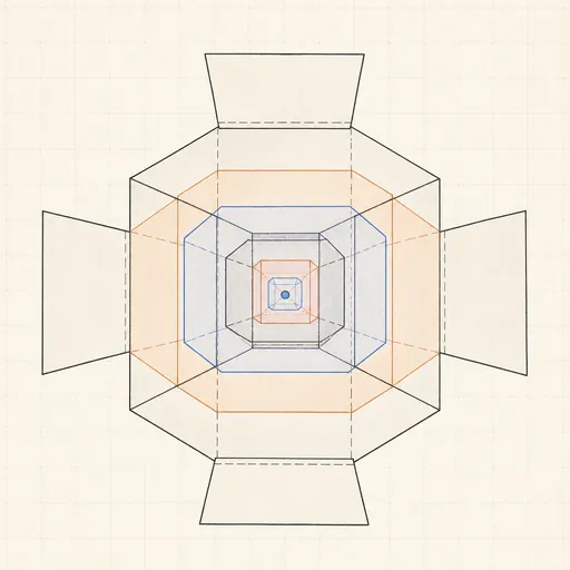
Watch distances concentrate and nearest neighbors fail as dimensions pile up.
Feature Scaling Demo
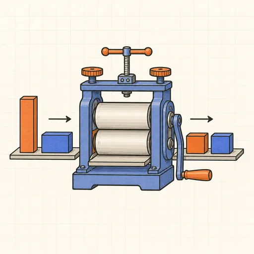
Run k-means and gradient descent on raw versus scaled features and watch scaling decide the outcome.