Conway's Game of Life, Explained
After reading this you will know the three rules that drive Conway's Game of Life, be able to compute the next generation of any pattern by hand, and understand why gliders, guns and blinkers arise from a grid that has no memory of its own past.
What the Game of Life is
The Game of Life is a cellular automaton invented by John Conway in 1970. It has no players and no goal. You set up a grid of square cells, mark some as alive, and then let a fixed rule decide the next state of every cell at once. That single step is called a generation. Repeat, and a pattern unfolds.
The rule looks at each cell and its eight touching neighbours (up, down, left, right, and the four diagonals). Nothing else matters: not the cell's age, not what happened three steps ago, not any global signal. Every cell reads its eight neighbours and updates simultaneously.
Here is the hook. Take a shape called the glider, five live cells in a diagonal arrow. Run it four generations and the identical shape reappears, shifted one cell down and one cell right. The pattern walks across the grid forever. Nothing in the rules mentions motion, yet motion emerges. That gap between trivial rules and rich behaviour is the whole point of the model.
When to use it, and when not
Use the Game of Life to see how local rules produce global structure. It is the standard first example of emergence, self-replication and undecidability made visible. If you want to feel why "simple rules, complex outcome" is a real phenomenon rather than a slogan, painting a few cells and pressing play does that in seconds.
Do not use it as a model of real biology. The name is a metaphor. Real cells do not update in lockstep on a fixed square lattice, and real populations do not die from having exactly one or four neighbours. The Game of Life is a mathematical object. Its value is that it is completely defined and completely deterministic, so any surprise you see comes from the rule alone and not from hidden noise.
The grid here is a torus: it wraps around at the edges. A glider that leaves the right edge reappears on the left. On a small grid this means a pattern can collide with its own output after wrapping, which changes the outcome compared to Conway's idealized infinite plane.
The rule stated precisely
Let s be the state of a cell, either 1 (alive) or 0 (dead). Let n be the number of its eight neighbours that are alive, so n ranges from 0 to 8. The next state s' is:
Read it as three plain statements. A live cell with 2 or 3 live neighbours stays alive. A dead cell with exactly 3 live neighbours becomes alive (birth). Every other cell ends up dead. Overcrowding (four or more neighbours) and isolation (zero or one neighbour) both kill.
You can compress the two survival-or-birth cases into one line. A cell is alive next step exactly when
This is why the rule is often labelled B3/S23: Born on 3, Survives on 2 or 3. Change those numbers and you get a different automaton with different creatures. Conway chose these values after testing many alternatives, because they balance growth against collapse: most patterns neither die out instantly nor explode without limit.
A worked example: the glider
Advancing the glider one generation by hand
Load the glider preset, the tool's default pattern. Place its five live cells at these coordinates, writing (column, row) with row increasing downward:
(1,0), (2,1), (0,2), (1,2), (2,2).
- Count neighbours for the cell at
(1,1), the empty centre. Its eight neighbours include(1,0),(2,1),(0,2),(1,2),(2,2): that is5live neighbours. It is dead with n = 5, so it stays dead. - Cell
(1,0)is alive. Its live neighbours are(2,1)and(1,2)?no,(1,2)is not adjacent to(1,0). Adjacent live cells are(2,1)only from the lower block plus none above, giving n = 1. With one neighbour it dies. - Cell
(2,1)is alive with live neighbours(1,0),(1,2),(2,2), so n = 3. It survives. - Empty cell
(0,1)has live neighbours(1,0),(0,2),(1,2), so n = 3. It is born. - Empty cell
(2,3)below the block has live neighbours(1,2),(2,2)and(2,1)?not adjacent. So n = 2, no birth. Empty cell(1,3)touches(0,2),(1,2),(2,2): n = 3, born.
Carry this out for every affected cell and generation 1 becomes (0,1), (2,1), (1,2), (2,2), (1,3). The population is still 5. After four such steps the arrow is identical to the start but moved one cell right and one cell down. Its speed is one cell diagonally per four generations, written c/4, where c is the fastest anything can move on the grid (one cell per step).
Reading the counters and the long run
The generation counter tells you how many update steps have run. The population counter tells you how many cells are alive right now. Watching population over time is the quickest way to classify a run.
A still life like the 2x2 block has constant population forever. A blinker oscillates: three cells in a row become three in a column and back, period 2, so its population stays at 3 but its shape flips. The pulsar preset has period 3. The R-pentomino, five cells, is famous for chaos: it churns for 1103 generations, throwing off six gliders, before settling into a still, oscillating debris field of 116 cells. The Gosper glider gun grows without bound, adding one glider every 30 generations, so its population climbs in a staircase.
Seed a random soup with the density slider and watch population fall fast, then flatten. From a dense start most cells die of overcrowding in the first few steps, then the survivors organize into still lifes and blinkers. The flat tail is the signature of a settled soup.
An experiment you can run: density versus survival
The single most instructive knob is the initial density: the fraction of cells you seed alive. Too sparse and everything dies of isolation. Too dense and everything dies of overcrowding. Somewhere in between the population survives longest and produces the most structure.
Run it at density 0.05 and the settled count is near 0. Run it at 0.375 and a 50 by 50 grid (2500 cells) tends to settle around 70 to 90 live cells, roughly 3 percent. Run it at 0.90 and almost everything dies within ten steps. The peak is broad and flat, not a sharp point, so any density between about 0.25 and 0.45 gives you a busy soup.
Common mistakes
The errors below all produce wrong generations by hand or wrong intuitions about the model.
- Updating cells one at a time
- The whole grid updates simultaneously from the current state. If you flip a cell and then count its neighbours for the next cell, you contaminate the count. Always compute all neighbour counts from the old grid, then apply them together.
- Counting only four neighbours
- The neighbourhood is the eight-cell Moore neighbourhood, including diagonals. Using the four-cell von Neumann neighbourhood gives a completely different automaton.
- Forgetting the birth rule
- A dead cell with exactly
3live neighbours comes alive. Beginners often track only survival and miss every birth, so their patterns shrink incorrectly. - Expecting the torus to match the infinite plane
- On this wrap-around grid a glider that would fly off forever instead returns and interferes. Small-grid results are not the canonical infinite-plane results.
Related tools on this site
The Game of Life is two-dimensional and updates on the Moore neighbourhood. For the one-dimensional cousin where each row depends on three cells above it, see the Elementary Cellular Automata tool, home of Rule 30 and Rule 110. Both models show complexity from tiny rules, and Rule 110, like Life, is Turing complete.
If you want emergent structure from a continuous rule rather than a discrete grid, the Mandelbrot Explorer generates infinite detail from a single iterated equation. And to see a different kind of build-up from parts, the Fourier Epicycles tool reconstructs any drawing from rotating circles.
Frequently asked questions
Why is it called a game if there are no players?
Conway used "game" loosely, as in a mathematical game with rules and outcomes. You choose the starting position, which is the only input. After that the rule plays itself with no further decisions.
Does every pattern eventually stop or repeat?
No. Some patterns grow forever. The Gosper glider gun emits one glider every 30 generations without limit, so its population increases without bound. Others, like the block, are fixed from the start.
Can the Game of Life compute anything?
Yes. Life is Turing complete. Using gliders as signals and guns as sources, people have built logic gates, memory and even working computers inside the grid. Anything a computer can compute can in principle be arranged as a Life pattern.
What is a glider gun?
A glider gun is a pattern that returns to its own shape on a period while releasing a glider each cycle. The Gosper gun has period 30 and was the first known pattern proving that populations in Life can grow forever.
Why do most random starts die down so quickly?
At high density many cells have four or more neighbours and die of overcrowding on the first step. The population usually drops by more than half within the first few generations, then the survivors settle into still lifes and blinkers.
Related tools
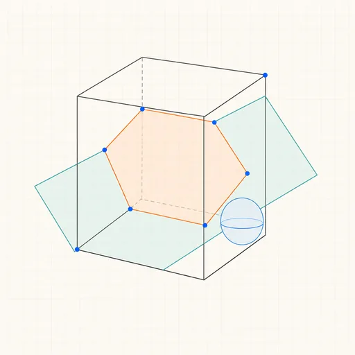
3D Geometry Board
Points, lines, planes, spheres and polyhedra on an orbiting camera — slice solids with planes, unfold nets, drop the Dandelin spheres into a cone and drag everything.
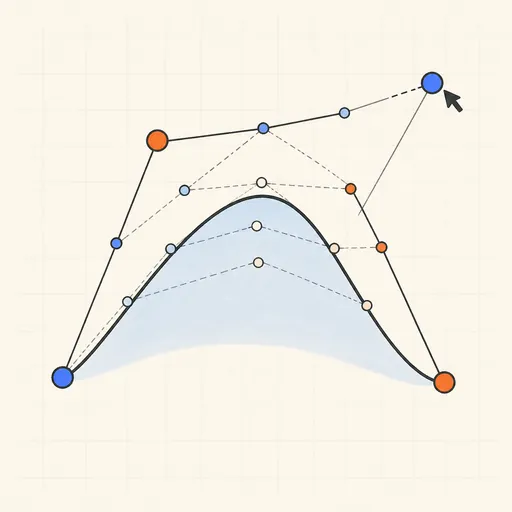
Bézier Curve Playground
Drag control points and watch De Casteljau’s algorithm construct a Bézier curve step by step.
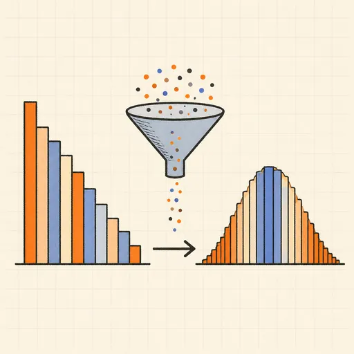
Central Limit Theorem Demo
Sample from any lopsided distribution and watch the averages pile up into a bell curve.
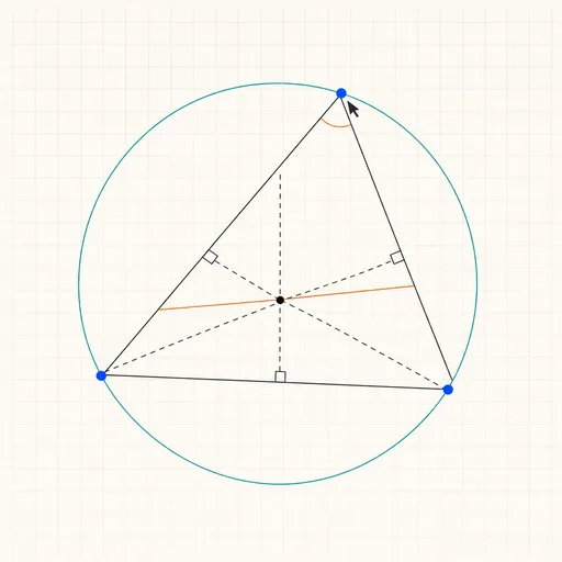
Dynamic Geometry Board
Construct with points, lines, circles and transformations, then drag anything — the construction stays true, and a checker tells you which relations are theorems.
Fantasy Map Generator
Roll a seed and get a continent: coastlines, mountains, rivers, biomes and named towns, ready for your campaign.
Fifteen Puzzle
Slide the tiles back into order — and learn the parity argument that makes half of all positions impossible.