How a Circuit Simulator Solves Your Circuit

After reading this you will understand how a circuit simulator turns a grid of components into a set of equations, solves them many times per second, and animates the current so you can read voltage, current and time constants directly off the screen.

What the simulator actually computes

A circuit simulator does not guess at current flow. It writes down the physical laws that every node and every branch must obey, then solves that system of equations for the one set of voltages and currents that satisfies all of them at once. On the grid you place a battery, a resistor and a wire loop; behind the scenes the tool builds a matrix, solves it, and reports that the current is, say, 0.5 amps everywhere in the loop.

Here is the hook. Connect a 9 V battery to a single 18 Ω resistor. Ohm's law says the current is I = V/R = 9/18 = 0.5 A. The simulator draws moving dots around the loop at a speed proportional to 0.5 A, and shades the wire from the battery's positive terminal (high voltage) to its negative terminal (low voltage). Change the resistor to 9 Ω and the current doubles to 1.0 A; the dots move twice as fast. Nothing here is animation for its own sake. Every visual maps to a number you can verify.

When to use it, and when not to

This tool is for building intuition about ideal analog circuits: how a voltage divider splits a voltage, how an RC pair sets a time constant, how a diode clips a waveform. It is fast, forgiving and local. You can short a battery and read a large current instead of destroying hardware.

It is not a replacement for a bench or for professional SPICE work. Components are ideal. Wires have zero resistance. Sources have no internal resistance. Nothing heats up, drifts with temperature, or burns out. If you need to know whether a real resistor will survive a fault, or how a trace's parasitic inductance rings at 100 MHz, this is the wrong tool. Use it to learn the model, then respect the gap between the model and a soldering iron.

The equations: modified nodal analysis

The solver uses modified nodal analysis (MNA). Start with Kirchhoff's current law: at every node, the currents flowing in equal the currents flowing out. For a resistor between nodes a and b, the current from a to b is the voltage difference divided by the resistance.

Here V_a and V_b are the node voltages, R is resistance in ohms, and G = 1/R is conductance in siemens. Writing KCL at every node using conductances gives a linear system:

G is the conductance matrix, \mathbf{v} is the vector of unknown node voltages, and \mathbf{i} is the vector of known currents injected at each node. Resistors alone would let you stop here. But a voltage source fixes a voltage difference and lets an unknown current flow, so KCL cannot express it directly. MNA fixes this by adding one extra unknown (the source current) and one extra equation (the source's voltage constraint) for each voltage source. The matrix grows a little, and the solve handles sources and resistors together in one shot.

Capacitors and inductors bring time into the problem. Their current depends on how voltage changes, not just its value:

C is capacitance in farads, L is inductance in henries. The simulator advances time in small steps of size \Delta t and replaces each capacitor with a resistor plus a current source (the backward-Euler companion model) whose values depend on the previous step. That keeps the whole system linear at each step and stable even with a large \Delta t. Diodes and LEDs are nonlinear, so the solver linearizes the Shockley equation and iterates with Newton's method until the operating point stops moving.

A worked voltage divider

Reading current, voltage and the RC charge curve

Wire color encodes node voltage: brighter or warmer shading means higher voltage relative to ground. Moving dots encode branch current: their speed scales with magnitude and their direction shows conventional current flow (from high to low potential through a resistor). A wire with no dots carries no current.

The most instructive time-domain circuit is the RC charge. Put a 9 V source, a switch, a resistor R and a capacitor C in series. When the switch closes, the capacitor voltage rises toward the source voltage on this curve:

The product \tau = RC is the time constant in seconds. With R = 1 kΩ and C = 100 µF, \tau = 1000 \times 0.0001 = 0.1 s. After one time constant the capacitor reaches 1 - e^{-1} = 0.632, so V_C = 9 \times 0.632 = 5.69 V. After five time constants (0.5 s) it reaches 9 \times 0.993 = 8.94 V, close enough to full charge that the dots nearly stop.

Common mistakes

Most confusing results come from a handful of setup errors, not from the solver.

No ground reference

MNA measures every voltage relative to a reference node. Without a ground, the system has no unique solution. Always place one ground.

Floating nodes

A wire connected at only one end, or a component leg left in the air, gives an undefined voltage there. Complete every loop.

Shorting a source

A bare wire across a battery reports a huge current. That is the ideal model telling you the resistance is zero, not a real reading.

Reading direction backward

Dots move in the direction of conventional current, from positive to negative outside the source. Electrons move the other way. The tool shows conventional current.

Diode polarity

An LED conducts only when forward biased. Reverse it and current stays near zero and the LED stays dark. Flip it if nothing lights.

Full-wave rectifier: reading a nonlinear result

Load the full-wave rectifier preset to see the Newton solver at work. A sine source drives four diodes in a bridge, so both halves of the input appear as positive output. An ideal silicon diode drops about 0.7 V when conducting, and the bridge always passes through two diodes in series, so the peak output is roughly the input peak minus 2 \times 0.7 = 1.4 V. Feed a 9 V peak sine and the rectified peaks reach about 7.6 V.

Add a capacitor across the output and the valleys fill in: the capacitor holds charge between peaks, so the trace flattens into rippled DC. The larger the capacitor, the smaller the ripple, because a bigger \tau discharges more slowly between peaks.

Related tools

If you like watching a solver step a physical model forward in time, these use the same idea in other domains. The Nuclear Reactor Simulator integrates neutron and xenon dynamics as you move control rods. The Bridge Builder & Truss Simulator solves a linear system for the force in every member, much like MNA solves for currents. The Orbital Mission Planner steps orbital mechanics to plan a transfer between planets.

Related tools

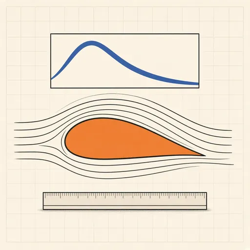
Airfoil Designer & Analyzer

Shape a NACA airfoil, see its pressure distribution and plot lift and drag polars, XFOIL-style, in the browser.

Bottle Rocket Simulator

Fill a soda-bottle water rocket, pump it up and launch it: find the water level, pressure and fins that fly highest.

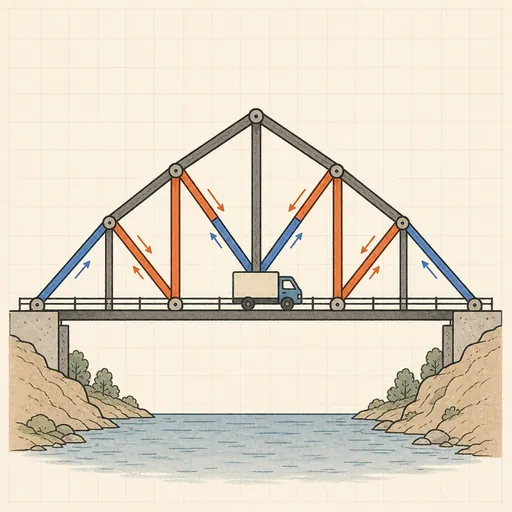
Bridge Builder & Truss Simulator

Design a truss bridge, send a truck across and watch every member strain, buckle or snap under load.

Earthquake Shake Table Simulator

Shake a multi-story building with an earthquake and watch it sway, crack or survive, with base isolation and dampers.

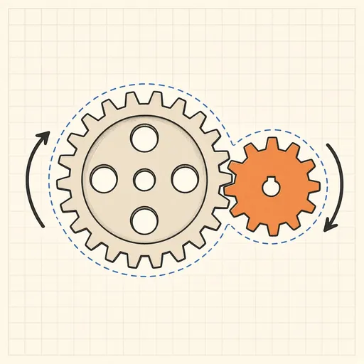
Gear Generator

Design involute spur gears, racks and planetary sets, watch them mesh and export SVG or DXF for laser cutting.

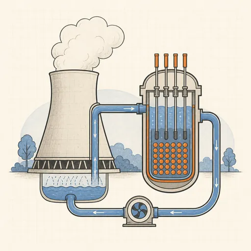
Nuclear Reactor Simulator

Run a pressurized-water reactor: pull control rods, manage xenon and temperature — or SCRAM before it overheats.