Brownian Motion, Explained
After reading this you will know why a large particle jitters in a fluid, how to predict the spread of its path from temperature and size, and how to read a mean squared displacement plot to extract a diffusion coefficient.
What Brownian motion is
Put a grain of pollen in water and watch it under a microscope. It never sits still. It jerks in one direction, then another, tracing a jagged path that never repeats. Robert Brown reported this in 1827 and could not explain it. The grain was not alive, and no current was stirring the water.
Albert Einstein gave the explanation in 1905. The water is made of molecules moving fast in every direction. They are far too small to see, but they hit the grain constantly. At any instant the hits from the left do not exactly cancel the hits from the right, so a small net force survives and shoves the grain a little. A moment later the imbalance points a different way. The grain gets pushed around by pure chance.
The simulation shows this directly. A single large tracer particle sits in a box of many small fast molecules. The molecules bounce off the tracer elastically. You never see a single collision decide the motion. Instead thousands of them add up, and the tracer wanders. The path it draws is a random walk: no memory of where it came from, no preferred direction.
When this model helps, and when it misleads
The model is a good picture of diffusion at small scales: a fluorescent bead in water, a smoke particle in still air, or a single protein drifting inside a cell. In all of these, a body far larger than the molecules around it moves only because of molecular buffeting.
The model is a poor picture whenever something other than random kicks dominates. If you blow on the smoke, that is convection, not diffusion, and the path gains a clear direction. If the tracer is charged and sits in a field, drift takes over. If the tracer is comparable in size to the molecules, the clean statistics below break down because a single collision matters.
This is a two dimensional toy. Real Brownian motion is three dimensional, and real molecules have a distribution of speeds set by the Maxwell-Boltzmann law rather than the single speed used here. The scaling laws survive that simplification, which is why the plots still look right.
The formula and the intuition behind it
A random walk does not go anywhere on average. Kicks left cancel kicks right, so the mean position stays near the start. What grows is the spread. The right measure is the mean squared displacement, written \langle r^2 \rangle: the average of the squared distance from the start, taken over many identical runs or many restarts.
Here \langle r^2 \rangle is the mean squared displacement in units of length squared, t is elapsed time, and D is the diffusion coefficient, a single number that says how fast the particle explores space. The factor 4 is specific to two dimensions. In one dimension it is 2, in three dimensions it is 6, always twice the number of dimensions.
Why is the growth linear in time and not in time squared? Because each step is independent. If you add n independent random steps, the variances add, so the squared distance grows like n, and n is proportional to time. Distance itself grows like \sqrt{t}. To go twice as far the particle needs four times as long.
Einstein connected D to the fluid through the relation below, which lets you read the size of atoms from a microscope.
Here k_B is Boltzmann's constant, T is absolute temperature, \eta is the fluid viscosity, and a is the tracer radius. Two facts fall straight out. Raise the temperature and D rises: hotter molecules kick harder. Enlarge the tracer and D falls: a bigger target both catches more of each kick and has more mass to move.
A worked example using the demo settings
Load the tool with its default settings and press the demo button. The tracer starts in the middle and begins to wander. Suppose you let it run and record the squared distance from the start at a few times, averaged over several restarts. The numbers below are what a clean run with a diffusion coefficient of D = 2.5 length units squared per second looks like.
Reading D off the plot
- Pick two times on the mean squared displacement plot: t_1 = 2 s and t_2 = 8 s.
- Read the MSD values. At t_1 the plot shows
20, at t_2 it shows80. - Compute the slope: (80 - 20) / (8 - 2) = 60 / 6 = 10 per second.
- Use \langle r^2 \rangle = 4 D t, so the slope equals 4D. Then D = 10 / 4 = 2.5 length units squared per second.
That recovers the value you put in. The whole point of the plot is that the slope is a direct, honest measurement of D, needing nothing but a ruler and two points.
Reading and interpreting the results
Two views tell you different things. The path shows the qualitative behavior: it should look jagged at every scale, with no straight runs and no return to a favorite spot. The MSD plot shows the quantitative behavior: it should climb as a straight line through the origin.
Watch how the settings change the slope. Raising temperature speeds up the molecules, so each kick is harder and the slope steepens. Adding molecules means more kicks per second, again steepening the line. Shrinking the tracer makes it both an easier target to move and a lighter one, so it wanders faster and the slope rises. Every one of these matches the sign predicted by D = k_B T / (6 \pi \eta a).
The table below shows the effect of doubling each input in turn, starting from a run with slope 10.
| Change | Direction of D | New slope 4D |
|---|---|---|
| Temperature doubled | up, roughly 2 times | 20 |
| Molecule count doubled | up, roughly 2 times | 20 |
| Tracer radius doubled | down, roughly half | 5 |
| Nothing changed | same | 10 |
Measure the slope from the middle of the plot, not the first second. Early on, the tracer has taken too few kicks for the average to settle, and the line is noisy. Fit a straight section well away from t = 0.
Common mistakes
The first mistake is reading a direction into the path. A run that happens to drift up and to the right for a while looks purposeful, but it is not. Over many restarts the average displacement is zero. Only the squared displacement grows, and it grows without any preferred direction.
The second mistake is expecting distance to grow at a steady rate. It does not. Because \langle r^2 \rangle = 4Dt, the typical distance is \sqrt{4Dt}, which grows like the square root of time. The particle covers ground quickly at first and then slows in its outward reach. It is not slowing down in speed, it is doubling back on itself.
The third mistake is treating a single run's MSD as exact. One path is one sample. The clean straight line appears only after averaging over many walkers or many restarts. A single noisy line with the right average slope is normal and correct.
Do not read absolute physical units off this toy. The length and time scales are arbitrary. What transfers to the real world is the shape of the laws: linear MSD, square-root spread, and the way the slope responds to temperature and size.
Related simulations to explore next
Brownian motion is randomness from many hidden causes. Chaos is a different route to unpredictability: fully deterministic yet wildly sensitive to starting conditions. See it in the Double Pendulum, where a rainbow swarm of nearby starts pulls apart within seconds.
For many bodies interacting under a real force law, try the Orbit Sandbox or the larger Galaxy Collision Simulator. To see collective molecular flow rather than single-particle jitter, stir the Fluid Flow Simulator, and to watch grains settle statistically, open the Falling-Sand Playground.
Frequently asked questions
Why does the tracer move if the molecular hits should cancel?
They cancel on average, not at every instant. At any moment the count of hits on one side differs slightly from the other by chance, so a small net force survives. That imbalance flickers direction constantly, which is exactly what produces a random walk.
Why is the mean squared displacement line straight instead of curved?
Each kick is independent of the last, so variances add over time. Adding n independent steps gives a squared distance proportional to n, and n is proportional to elapsed time. That is why \langle r^2 \rangle = 4Dt is linear.
What does the diffusion coefficient actually measure?
It measures how quickly the spread of positions grows. A D of 2.5 means the mean squared displacement climbs by 4 \times 2.5 = 10 length units squared every second. Double D and the particle explores twice the area in the same time.
How did Einstein use this to size atoms?
He measured D from the drift of visible particles, then inverted D = k_B T / (6 \pi \eta a) to get k_B, and from that Avogadro's number and the scale of molecules. Jean Perrin did the experiments and won the 1926 Nobel Prize for confirming atoms exist.
Why do bigger particles wander less?
A larger radius appears in the denominator of the Einstein relation, so D falls roughly as one over the radius. A bigger target is also heavier, and the same net kick moves a heavier body less. Both effects slow the wander.
Related tools
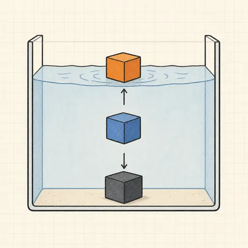
Buoyancy Tank
Drop blocks of different density into water and watch Archimedes decide what floats, sinks or hovers.
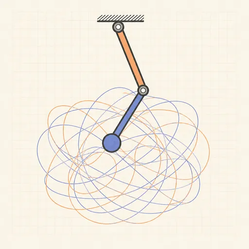
Double Pendulum
Swing a chaotic double pendulum and split it into a rainbow swarm to watch nearby starts diverge.
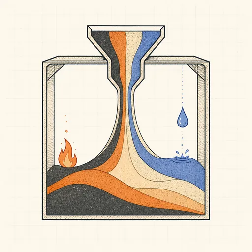
Falling-Sand Playground
Paint sand, water, oil, fire and more and watch them pour, settle, burn and react pixel by pixel.

Fluid Flow Simulator
Stir glowing dye through a real-time GPU fluid simulation.
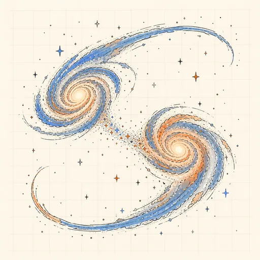
Galaxy Collision Simulator
Smash two spiral galaxies together and watch tidal tails and bridges form.
Hear the Shape of a Drum
Draw any drum and hear its true vibration modes — then meet two different drums that sound exactly the same.