Word Embeddings from Skip-Gram, Explained
After reading this you will know how word2vec turns words into vectors, how skip-gram with negative sampling trains those vectors with a simple logistic loss, and how to read the clusters, neighbours and analogies the trainer produces.
What word embeddings are
A word embedding is a fixed-length list of numbers assigned to a word. If you pick an embedding dimension of 50, then the word dog becomes a point in 50-dimensional space, something like [0.14, -0.62, 0.03, ...] with 50 entries. The numbers are learned, not chosen. Words that appear in similar contexts end up near each other in that space.
Here is the hook. Train on enough text and the vector for Paris minus France plus Italy lands close to Rome. The offset from a country to its capital becomes roughly the same direction for every country pair. That is not magic. It is a side effect of one training rule applied millions of times, which the next sections spell out with numbers.
The core idea, from Mikolov and colleagues in 2013, is that you learn word meaning from company. A word is defined by the words that surround it. Train a tiny model to predict neighbours from a center word and the weights of that model become the embeddings.
When to use this, and when not
Skip-gram embeddings are useful when you have a lot of raw text and want a compact numeric representation of each word for a downstream task: clustering, similarity search, or feeding a small classifier. They need no labels. They capture co-occurrence patterns, which cover a surprising amount of what people call meaning.
They are the wrong choice in three cases. First, when word order and long-range structure matter, because a single vector per word ignores position; the Self-Attention Visualizer shows the mechanism modern models use instead. Second, when a word has several senses, since bank collapses to one vector blending river and money. Third, when your corpus is tiny. A few kilobytes of text give rough, noisy embeddings. The clusters on screen will look plausible, but the exact distances shift every run.
Treat the browser trainer as a teaching instrument, not a production pipeline. Published embeddings are trained on billions of tokens across many hours. A textarea holds a few thousand tokens and trains in seconds. You will see related words drift together, but do not expect stable king minus man plus woman results at this scale.
The formula and the intuition
Skip-gram uses two vectors per word: an input vector v_w when the word is the center, and an output vector u_w when the word is a context. For a center word c and a true context word o, the model scores the pair by a dot product and squashes it with the logistic function.
Here u_o \cdot v_c is the dot product of the context vector and the center vector, a single number. \sigma is the sigmoid. When the dot product is large and positive the probability is near 1; when it is large and negative the probability is near 0. See the Activation Function Explorer for how sigmoid behaves.
Training the full softmax over the whole vocabulary V costs O(V) per update. Negative sampling avoids that. For each real pair it draws k fake context words and asks the model to score them low. The loss for one center-context pair becomes:
The first term pushes the real pair score up. Each term in the sum pushes a negative pair score down, because \sigma(-x) = 1 - \sigma(x). The negatives n_i are drawn from the unigram distribution raised to the 3/4 power, which pulls sampling toward rare words compared to raw frequency.
Here f(w) is the raw count of word w. The 3/4 exponent is a tuned constant: it damps very frequent words like the without ignoring them entirely.
A worked example you can check by hand
One gradient step on a two-dimensional embedding
Use dimension 2 so every vector fits on paper. Suppose after some training you have these vectors, and you process the true pair center cat, context dog with one negative the.
- Center vector v_{cat} = [0.5, -0.2]. Context vectors u_{dog} = [0.4, 0.1] and u_{the} = [-0.3, 0.6].
- Positive score: u_{dog} \cdot v_{cat} = 0.4(0.5) + 0.1(-0.2) = 0.20 - 0.02 = 0.18. Then \sigma(0.18) = 0.5449.
- Negative score: u_{the} \cdot v_{cat} = -0.3(0.5) + 0.6(-0.2) = -0.15 - 0.12 = -0.27. Then \sigma(-0.27) = 0.4329, so this negative is already scored fairly low.
- Loss: -\log(0.5449) - \log(0.4329) = 0.6070 + 0.8374 = 1.444.
- Gradient signal for the positive pair is \sigma(0.18) - 1 = -0.4551. For the negative it is \sigma(-0.27) applied as \sigma(u_{the}\cdot v_{cat}) = 0.5671 times the update direction.
- Update u_{dog} with learning rate
0.1: gradient is (\sigma(0.18)-1)\,v_{cat} = -0.4551 \times [0.5,-0.2] = [-0.2276, 0.0910]. New u_{dog} = [0.4,0.1] - 0.1[-0.2276,0.0910] = [0.4228, 0.0909].
The context vector for dog moved toward cat. Repeat this over every window in the corpus and words that share neighbours converge. The mechanics are ordinary gradient descent, the same loop shown number by number in Backpropagation Step-by-Step.
0.18 (score 0.5449) and -0.27 (score 0.4329). Training pushes real pairs right and negatives left.Reading the map, neighbours and analogies
The embedding space has many dimensions, so the tool shows a PCA projection onto two axes. PCA finds the plane of maximum variance and drops everything else. Two words that look close on screen may be farther apart in the full space, and words that look far apart on screen might share a direction PCA discarded. Trust the neighbour list, which uses full cosine similarity, over the picture.
Cosine similarity is the angle between two vectors, ignoring length:
A value near 1 means the vectors point the same way, near 0 means unrelated, near -1 means opposite. For the analogy row, the tool computes v_a - v_b + v_c and returns the word whose vector has the highest cosine similarity to that result, excluding the three input words.
| Cosine | Angle | Reading |
|---|---|---|
| 1.000 | 0° | Same direction, strongest neighbour |
| 0.7071 | 45° | Clearly related |
| 0.000 | 90° | Unrelated |
| -0.500 | 120° | Pointing away, rare in practice |
Common mistakes
The frequent errors are practical, not conceptual.
- Too little text
- With a few hundred words, most pairs appear once or twice. Vectors barely move, and the map reshuffles each run. Paste more text before drawing conclusions.
- Reading the 2-D plot as truth
- PCA discards dimensions. If the neighbour list disagrees with the picture, the neighbour list is right, because it uses the full vectors.
- Window too wide
- A context window of
10on short informal text mixes unrelated words into every center. Topic-level similarity blurs. Windows of2to5keep neighbours syntactically tight. - Expecting stable analogies
- The analogy trick needs consistent relations repeated many times. In a few kilobytes the offset vectors are noisy, so
king - man + womanoften returns a frequent word rather thanqueen. - Confusing the two vector sets
- Each word has an input and an output vector. Similarity is computed on the input vectors. Do not mix them.
If clusters look random, raise the epoch count and the amount of text before touching dimension or window. More passes over more data help far more than a larger embedding size on a small corpus.
How the pieces fit the wider toolkit
Skip-gram is a shallow network trained by gradient descent, so the same ideas appear across these tools. To see gradient descent shape a decision boundary, try the Neural Network Playground. To watch gradients grow or shrink through many layers, the reason deep models were once hard to train, see Vanishing & Exploding Gradients. To keep weights from overfitting a small corpus, the shrinkage in the Regularization Demo uses the same penalty families. For a model that reads text one symbol at a time, the Character RNN Text Generator is a natural next step, and for image data the Convolution Filter Visualizer shows the convolution equivalent of local context.
Frequently asked questions
Why two vectors per word instead of one?
Skip-gram keeps a separate input vector for the center role and output vector for the context role. This makes the dot products asymmetric and the math cleaner. Most implementations report the input vectors as the embeddings, or average the two.
What does the loss number tell me?
It is the average negative log likelihood over recent pairs, like the 1.444 computed for one pair above. A falling loss means real pairs score higher and negatives score lower. It will not reach zero, because words are genuinely ambiguous.
Why raise the unigram counts to the 3/4 power?
Raw frequency oversamples words like the as negatives. The 3/4 exponent compresses the gap: a word appearing 1000 times gets weight 1000^{0.75} \approx 178, while one appearing 10 times gets 10^{0.75} \approx 5.6, a ratio of 32 rather than 100.
How large should the embedding dimension be?
For a textarea corpus, 20 to 50 is plenty. Higher dimensions need more data to fill meaningfully. Published models use 100 to 300 trained on billions of tokens.
Why do results change every time I train?
Vectors start from random values, negatives are sampled randomly, and PCA can flip axis signs. The clusters are stable up to rotation and reflection, but exact coordinates and the sign of an axis will vary between runs.
Related tools
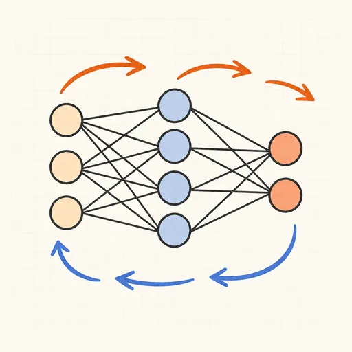
Backpropagation Step-by-Step
Walk through one forward and backward pass of a tiny neural network, number by number.

Handwritten Digit Recognizer
Draw a digit and watch a neural network trained on MNIST recognize it live in your browser.
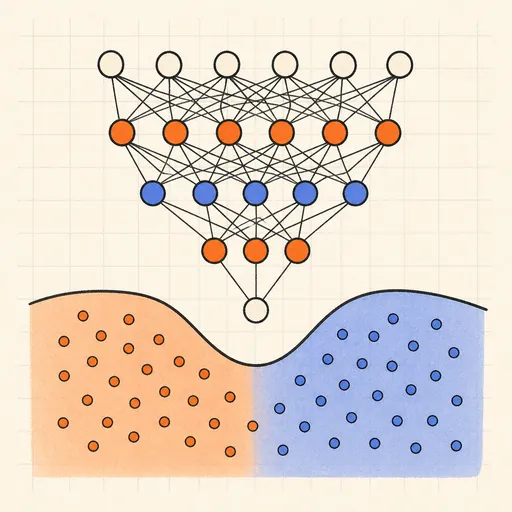
Neural Network Playground
Train a tiny neural network live in your browser and watch its decision boundary learn four classic datasets.

Activation Function Explorer
Compare sigmoid, tanh, ReLU and friends with their derivatives, and see why deep gradients vanish.
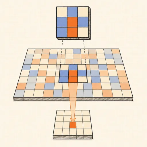
Convolution Filter Visualizer
Slide a 3×3 kernel over an image and watch convolution, ReLU and max-pooling build the output pixel by pixel.

Hopfield Network
Store pixel patterns in a Hopfield memory, corrupt them, and watch the network recall the original.