Overfitting, Explained
After reading this you can tell underfitting from overfitting by eye and by number, derive why test error is U-shaped in a polynomial's degree, and pick the degree that generalizes best on noisy data.
What overfitting is, and one picture that shows it
Overfitting happens when a model learns the noise in its training data instead of the signal. You see it most clearly when you fit polynomials of increasing degree to a few noisy points. A degree-1 line is too stiff to bend toward the true curve. A degree-15 polynomial is so flexible it threads every training point exactly, then swings violently between them.
The Overfitting Sandbox draws this directly. It samples a hidden function (sine, step, or cubic), adds Gaussian noise, splits the points 70/30 into training and test sets, and fits a polynomial of your chosen degree by least squares. Filled dots are training points; hollow dots are test points held out from the fit. As you raise the degree, the fitted curve gets closer to every filled dot and further from the dashed truth in between.
The key fact: fitting the training points well is not the goal. The goal is predicting points the model has never seen. Those two things agree at low degree and disagree sharply at high degree.
The bias-variance tradeoff behind the curves
Expected test error at a point decomposes into three parts. Write the true function as f(x), the noisy observation as y = f(x) + \varepsilon with noise variance \sigma^2, and the model's prediction as \hat{f}(x). Then:
Bias is how far the average fitted curve sits from the truth. A low-degree polynomial has high bias: it simply cannot match a wiggly target. Variance is how much the fit jumps around when you resample the training data. A high-degree polynomial has high variance: shift one point and the curve reshapes wildly. The last term \sigma^2 is irreducible noise, the floor no model can beat.
As degree grows, bias falls and variance rises. Test error is their sum plus the floor, so it drops, bottoms out, then climbs. That is the U shape. Training error, by contrast, only ever falls (weakly) as degree grows, because more flexibility can only fit the training points better.
The noise floor is a hard limit. If the truth is a sine with \sigma = 0.2, then \sigma^2 = 0.04. No polynomial, at any degree, will reliably push test MSE below 0.04. Chasing lower test error than the floor means you are fitting noise.
The least-squares fit and why the basis matters
For a degree-d polynomial, the model is \hat{y} = \sum_{j=0}^{d} w_j \phi_j(x). Stack the basis values into a design matrix X with one row per training point. Least squares picks the weights that minimize squared error:
Here y is the vector of training targets and \hat{w} the fitted coefficients. The mean squared error you read off the charts is
with n the number of points in whichever split you are scoring, train or test.
The basis choice is not cosmetic. If you use raw powers 1, x, x^2, \dots, x^{15}, the columns of X become nearly parallel and X^\top X turns catastrophically ill-conditioned. The sandbox fits on a Chebyshev basis over [-1, 1] instead, whose columns stay nearly orthogonal, so the normal equations stay solvable at degree 15.
A worked example on the demo data
Press the demo button, which uses the field defaults, and you can reproduce the arithmetic below on a small slice. Suppose five training points are drawn from a cubic truth with mild noise:
Fitting five points by hand
Take these training points and fit a horizontal line (degree 0), which just predicts the mean.
| x | y |
|---|---|
| -0.8 | -0.30 |
| -0.4 | 0.10 |
| 0.0 | 0.05 |
| 0.4 | 0.20 |
| 0.8 | 0.55 |
- Degree 0 predicts the mean of
y: \bar{y} = (-0.30 + 0.10 + 0.05 + 0.20 + 0.55)/5 = 0.12. - Training MSE is the average squared gap from
0.12: the squared errors are0.1764,0.0004,0.0049,0.0064,0.1849. - Their average is \text{MSE}_{\text{train}} = 0.3730/5 = 0.0746. This is high because a flat line cannot follow the upward trend: that is bias.
- Now fit degree 1 (a straight line). Least squares gives slope near
0.50and intercept near0.12. The line tracks the trend, so training MSE drops to about0.0100. - Fit degree 4 through these five points and the polynomial passes through all of them exactly: training MSE is
0. A degree-n polynomial interpolates n+1 points exactly.
Zero training error at degree 4 looks perfect. It is not. Those wiggles between the points chase the noise, so on held-out test points the same degree-4 fit scores far worse than the honest degree-1 line.
An explorer for the U-shaped curve
The static chart below shows a typical sweep. The interactive lets you move the pieces that produce the U so you can watch bias fall and variance rise separately.
Reading the verdict and choosing a degree
Compare the two numbers, not one alone. Three patterns cover almost every case:
- Underfit
- Both train and test MSE are high and close together. Example: degree 1 on a sine gives train
0.31and test0.31. The model is too stiff. Raise the degree. - Good fit
- Test MSE is near its minimum and close to the noise floor, with a small gap above training MSE. Example: degree 5 gives train
0.030, test0.047, floor0.04. Stop here. - Overfit
- Training MSE is tiny but test MSE is large and rising. Example: degree 14 gives train
0.005and test0.90. The gap between the two is the tell.
The practical rule: pick the degree at the bottom of the test curve. If two nearby degrees tie, prefer the smaller one. A simpler model that scores the same is more robust to new data.
Common mistakes
Do not judge a model by training error. A degree-15 fit can drive training MSE to near zero while test MSE is 20 times worse. Low training error alone tells you the model memorized the sample, not that it learned the pattern.
Three more traps show up constantly. First, expecting test error below the noise floor. If \sigma = 0.3, then \sigma^2 = 0.09, and a test MSE of 0.09 is already optimal. Trying to beat it means fitting randomness.
Second, ignoring sample size. Variance in the tradeoff scales roughly like (d+1)/n. With n = 20 points a degree-10 fit has 11 parameters and almost no data per parameter, so it overfits early. With n = 200 the same degree behaves far better and the U shifts right.
Third, reading one random split as truth. The 70/30 split is one draw. Resample and the exact sweet-spot degree can shift by one or two. Cross-validation averages over many splits to reduce that wobble.
Related tools
Overfitting is not unique to polynomials. To see least squares fit a straight line and watch gradient descent move across the loss surface, use the Linear Regression Playground. To watch shallow trees stacked on residuals sharpen a 1D curve and then overfit exactly as high-degree polynomials do, see Gradient Boosting Step-by-Step. To see how bagging many randomized trees smooths a jagged, overfit boundary into a stable one, try Random Forest Voting. For a model whose single parameter k controls the same flexibility tradeoff (small k overfits, large k underfits), explore the k-Nearest Neighbors Explorer.
Frequently asked questions
Why does training error keep falling as degree increases?
More flexibility can only help fit the points already seen. Adding a term never makes the least-squares training error worse, and usually lowers it. Once degree reaches n-1 for n training points, the polynomial passes through every point and training MSE hits zero.
How do I know the true best degree if I only have data?
You do not measure it directly; you estimate it from held-out data. The hollow test points here do that job. In practice, use k-fold cross-validation and pick the degree with the lowest average validation error.
Can regularization fix overfitting without lowering the degree?
Yes. Adding a penalty like \lambda \lVert w \rVert^2 (ridge regression) shrinks large coefficients, which tames the wild swings of high-degree fits. You keep the flexible basis but constrain how aggressively it uses it. This sandbox uses plain least squares with no penalty, so degree is your only knob.
Why Chebyshev polynomials instead of plain powers?
Raw powers x^{12}, x^{13}, x^{14} are nearly identical over [-1,1], so the design matrix columns become collinear and the normal equations blow up numerically. Chebyshev basis functions stay nearly orthogonal, keeping X^\top X well-conditioned even at degree 15. The fitted curve is the same polynomial; only the arithmetic is stable.
Does more data always prevent overfitting?
More data raises the degree at which overfitting sets in, because variance scales like (d+1)/n. With enough points a high-degree fit can generalize well. But no amount of data beats the noise floor \sigma^2, and a model too simple to represent the truth stays biased no matter how many points you feed it.
Related tools
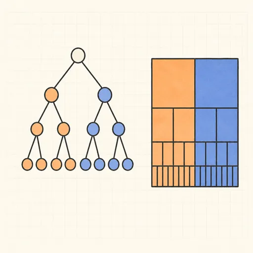
Decision Tree Builder
Grow a CART decision tree split by split and watch the partition map and tree diagram build together.
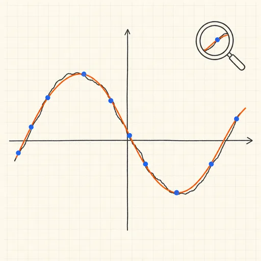
Function Sketch Finder
Sketch a curve on a zoomable coordinate grid and search dozens of function families for the equations that fit it best.
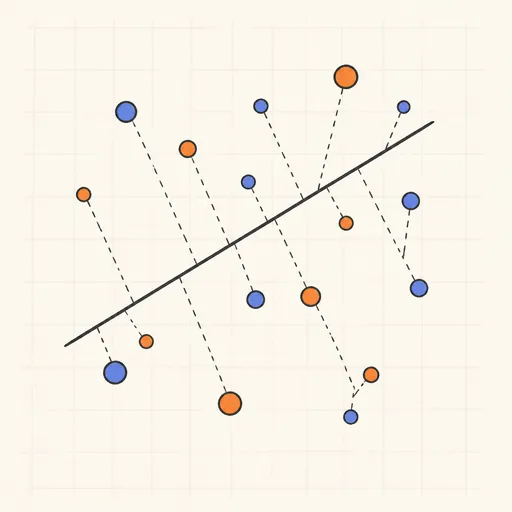
Linear Regression Playground
Place points, watch the least-squares line follow, and see gradient descent crawl across the loss surface.
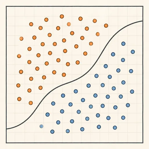
Logistic Regression Playground
Paint two classes of points and watch logistic regression carve out its probability boundary by gradient descent.

Naive Bayes Classifier Demo
Score your own message with a word-count spam filter, or watch Gaussian naive Bayes classify 2D points.
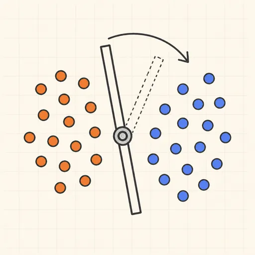
Perceptron Learning Animation
Step through Rosenblatt’s 1958 learning rule and watch the decision boundary rotate with every mistake.