The Neural Network Playground, Explained
After reading this you will understand how a small multilayer perceptron turns raw coordinates into a curved decision boundary, how backpropagation adjusts its weights, and how to read the train/test loss gap to spot overfitting.
What the playground does
The tool trains a tiny neural network to separate two classes of points on a flat 2-D plane. Each training point has two features, its x and y coordinates, and one label, blue (class 0) or orange (class 1). The network learns a function that maps every point on the plane to a probability of being orange, and the canvas paints that function as a heatmap.
Here is the hook. Take the XOR dataset: blue points sit in the top-left and bottom-right quadrants, orange in the top-right and bottom-left. No straight line can separate them. A network with zero hidden layers will fail, hovering near 50 percent accuracy forever. Add one hidden layer of four tanh neurons and within a few hundred epochs the boundary bends into a clean cross shape. The nonlinearity is what makes the bend possible.
When a neural network helps, and when it does not
A multilayer perceptron earns its keep when the boundary between classes is curved or made of several disconnected pieces. The concentric-circles and spirals datasets are exactly this: no line works, but a network with enough hidden units wraps the boundary around the shape.
When the two classes are already linearly separable, like two well-spaced gaussian blobs, a network is overkill. Logistic regression (a network with no hidden layer) draws a straight line and reaches near-perfect accuracy. Adding hidden layers there only gives the model more ways to chase label noise.
More neurons is not always better. On a linearly separable blob with 20 percent label noise, a three-layer network with eight neurons per layer will contort its boundary to fit noisy points, and its test loss will climb while its train loss keeps falling. That gap is overfitting, and you can watch it open in the loss chart.
The math: forward pass and loss
Each neuron computes a weighted sum of its inputs, adds a bias, then applies an activation function. For a single hidden layer with input vector x = (x_1, x_2), the value of hidden neuron j is:
Here w_{ji} is the weight from input i to neuron j, b_j is that neuron's bias, and \phi is the activation (tanh, ReLU or sigmoid). The output neuron takes the hidden values and applies a sigmoid to squash the result into a probability:
The v_j are the output weights, c is the output bias, and \hat{y} is the predicted probability of orange. To measure error the tool uses binary cross-entropy, averaged over the batch of N points:
When the true label y_n is 1 and the model predicts \hat{y}_n = 0.9, the loss for that point is -\ln(0.9) \approx 0.105. Predict 0.5 and it costs -\ln(0.5) \approx 0.693. Predict a confident wrong 0.1 and it costs -\ln(0.1) \approx 2.303. Confident mistakes are punished hard.
How backpropagation updates the weights
Training means nudging every weight in the direction that lowers L. The gradient of the loss with respect to each weight comes from the chain rule, applied layer by layer from output back to input. That backward sweep is backpropagation.
For the sigmoid output trained on cross-entropy, the algebra collapses to something clean. The error signal at the output is simply the prediction minus the target:
The gradient for output weight v_j is \delta \cdot h_j, and for the bias it is just \delta. To reach a hidden weight, you push \delta back through v_j and multiply by the activation's derivative. Each weight then moves against its gradient, scaled by the learning rate \eta:
The tool runs this in minibatches of 10 points at a time, which is why it is called minibatch stochastic gradient descent. If you want to see every number in one full pass by hand, work through Backpropagation Step-by-Step.
Weights start small and random, scaled by the fan-in of each layer: standard deviation \sqrt{1/n} for tanh and sigmoid, or \sqrt{2/n} for ReLU, where n is the number of inputs to the neuron. This keeps the initial signal from shrinking or blowing up as it passes through layers.
A worked example on the XOR dataset
One update step by hand
Use the demo defaults: the XOR dataset, one hidden layer, tanh activation. Take a single point at x = (1, 1) with true label orange, so y = 1. Suppose after initialization the network already produces hidden value h_1 = 0.6 and the output pre-activation is z = 0.2. Use learning rate \eta = 0.1.
- Forward: \hat{y} = \sigma(0.2) = 1/(1 + e^{-0.2}) \approx 0.5498.
- Loss for this point: -\ln(0.5498) \approx 0.598.
- Output error: \delta = \hat{y} - y = 0.5498 - 1 = -0.4502.
- Gradient for output weight v_1: \delta \cdot h_1 = -0.4502 \times 0.6 = -0.2701.
- Update: v_1 \leftarrow v_1 - 0.1 \times (-0.2701) = v_1 + 0.02701.
The weight moves up by 0.027, which raises the next prediction toward 1. Repeat over thousands of points and the boundary settles into the XOR cross.
Reading the heatmap and the loss curves
The canvas colours every pixel by the network's output there: deep orange means \hat{y} near 1, deep blue near 0, and pale colours near the 0.5 boundary. The pale band traces the decision boundary. Solid dots are training points, hollow dots are test points held out from training.
The second chart shows two loss numbers per epoch. When both fall together and stay close, the model is learning a pattern that generalizes. When train loss keeps dropping but test loss flattens then rises, the network is memorizing training points instead of the underlying shape. A useful rule of thumb: if test loss is more than roughly 1.5 times train loss and climbing, stop and shrink the network.
Common mistakes
- Learning rate too high
- Set \eta to
1.0and the loss often jumps around or shoots to infinity instead of settling. The weight update overshoots the minimum every step. If loss diverges, cut the learning rate by a factor of ten. - No hidden layer for a nonlinear problem
- A network with no nonlinear hidden layer can only draw a straight line. On XOR, circles or spirals it is stuck near 50 percent accuracy no matter how long it trains.
- Sigmoid in deep hidden layers
- Stack three hidden layers of
sigmoidunits and gradients shrink as they travel backward, so early layers barely move. The Vanishing & Exploding Gradients demo shows this per layer, and the Activation Function Explorer shows why: the sigmoid derivative peaks at just 0.25. - Reading accuracy off the training points only
- A boundary that threads perfectly between solid dots can still misclassify the hollow test dots. Judge the model by test loss, not the picture on training data.
Related tools
To fight the overfitting you see here, the Regularization Demo shows how L2 shrinks weights, L1 zeros them out, and dropout smooths the boundary. For a different network shape, the Convolution Filter Visualizer builds up image features with kernels, and the Handwritten Digit Recognizer applies a trained network to real MNIST digits you draw.
For networks that handle sequences and language, see the Character RNN Text Generator, the Self-Attention Visualizer, the Word Embedding Trainer, and the associative-memory Hopfield Network.
Frequently asked questions
Why does XOR need a hidden layer but the blobs do not?
Two gaussian blobs can be split by a single straight line, which is all a no-hidden-layer network can draw. XOR needs the boundary to turn, and only a nonlinear hidden layer lets the network combine several lines into a bent shape.
How many neurons do the spirals need?
The two interleaved spirals are the hardest of the four datasets. One hidden layer of four neurons usually fails. Try two hidden layers of six to eight tanh neurons, and give it several hundred epochs. The boundary has to coil, which needs many folds.
Why does my loss sometimes explode to a huge number?
Almost always the learning rate is too high. Each step overshoots and the weights grow without bound until the loss overflows. Lower the learning rate, then press Reset to re-roll the weights and start clean.
Does this scale to real problems?
The mechanics scale, but the size does not. This is a toy with two input features and a handful of neurons, trained on a few hundred points in your browser. Production networks have millions of parameters, many input dimensions, and specialized architectures. The value here is watching the exact algorithm that those large systems still use.
Why are some points hollow?
Hollow points are the test set, held out from training. The network never adjusts its weights to fit them, so how well the heatmap matches the hollow points tells you whether the model generalizes or has only memorized the solid training points.
Related tools
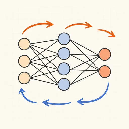
Backpropagation Step-by-Step
Walk through one forward and backward pass of a tiny neural network, number by number.

Handwritten Digit Recognizer
Draw a digit and watch a neural network trained on MNIST recognize it live in your browser.
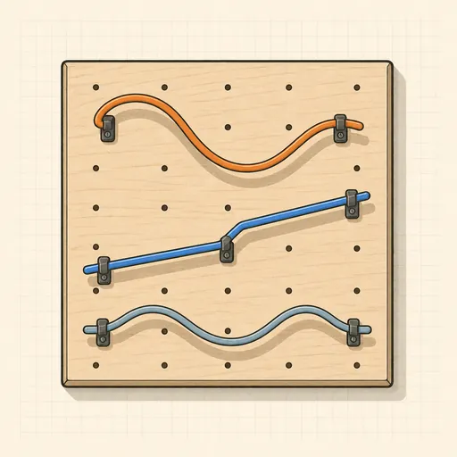
Activation Function Explorer
Compare sigmoid, tanh, ReLU and friends with their derivatives, and see why deep gradients vanish.
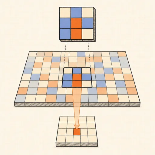
Convolution Filter Visualizer
Slide a 3×3 kernel over an image and watch convolution, ReLU and max-pooling build the output pixel by pixel.
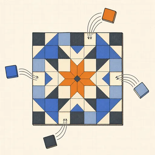
Hopfield Network
Store pixel patterns in a Hopfield memory, corrupt them, and watch the network recall the original.
Self-Attention Visualizer
See how Transformer tokens attend to each other with arcs, heatmaps, heads and causal masks.