Character RNN Text Generator, Explained
After reading this you will understand how a recurrent neural network predicts one character at a time, how it learns from a plain block of text, and how to read its loss curve and sampled output without fooling yourself about what a browser-sized model can do.
What a character RNN does
A character RNN is a next-character predictor. You feed it one character, it outputs a probability for every possible next character, you pick one, feed that back in, and repeat. Nothing in the model knows what a word is. It only ever sees single symbols and a hidden state vector that summarizes what it has read so far.
Here is the hook. Train the model on a page of English prose and watch its sampled output over time. At iteration 0 you get noise like qx,;jZ f9k. After a few hundred iterations spaces and common letters appear: the an to hes. After a few thousand iterations you get plausible-looking words and correct punctuation, even short phrases that read like the source, all from a model that never saw a dictionary. The structure of the language was recoverable from character statistics alone.
The Word Embedding Trainer works at the level of whole words. A character RNN works one level below that, which is why it can invent spelling and why it can handle any alphabet up to 96 distinct symbols without changes.
When to use it, and when not
Reach for a character RNN when you want to see sequence learning happen from scratch, with a model small enough to train live and inspect. It is a teaching model. The whole point is that you can watch the loss fall and the samples improve in real time.
Do not read production quality into it. This is a single-layer vanilla tanh RNN with a 25-character memory window. Real text generators use Transformers with attention over thousands of tokens, trained on billions of characters across many machines. The Self-Attention Visualizer shows the mechanism that replaced RNNs for long-range dependencies. If you need coherent paragraphs, a browser RNN is the wrong tool. If you want to understand why sequence models work at all, it is a good one.
The 25-character truncation is a hard limit on memory. If your training text depends on structure longer than 25 characters (matching quotes 40 characters apart, say), the model cannot learn that link no matter how long you train. The gradient that would teach it is literally cut off.
The forward pass and the update rule
Represent each character as a one-hot vector x_t: a vector of zeros with a single 1 at the character's index in the vocabulary. The hidden state updates at every step:
Here h_t is the hidden state (a vector of size equal to the hidden-layer setting), W_{xh} maps the input character into hidden space, W_{hh} carries the previous hidden state forward, and b_h is a bias. The \tanh squashes every hidden unit to the range (-1, 1). Compare its shape to the alternatives in the Activation Function Explorer.
To predict the next character, score every vocabulary symbol with a linear layer and turn scores into probabilities with a softmax:
The vector y_t holds one raw score (a logit) per vocabulary symbol. Dividing by temperature T reshapes the distribution before sampling, which we return to below. Training uses T = 1.
The loss is cross-entropy: the negative log probability the model assigned to the character that actually came next.
Gradients flow back through the unrolled network (truncated backpropagation through time), get clipped to the range [-5, 5] to stop them exploding, and each weight is updated by Adagrad, which divides the step by the root of that weight's accumulated squared gradient:
Weights with a history of large gradients take smaller steps, so different weights adapt at different rates. The clipping and the RNN's tendency to blow up are the exact subject of the Vanishing and Exploding Gradients demo.
A worked example you can check by hand
Loss on a four-character vocabulary
Suppose the corpus uses only the characters h, e, l, o, so the vocabulary size is 4. Before any training the model is roughly uniform over these 4 symbols.
- A uniform guess assigns probability
1/4 = 0.25to the correct next character. - The per-character loss is -\ln(0.25) = 1.386. That is the starting loss you should expect for a 4-symbol vocabulary.
- Now say training raises the probability of the correct character to
0.60. The loss drops to -\ln(0.60) = 0.511. - The theoretical floor is -\ln(1.0) = 0, reached only if the model is perfectly certain and always right, which never happens on real text.
The general rule: a model that has learned nothing sits near \ln(V) where V is the vocabulary size. For a typical English corpus with V \approx 50 distinct symbols, expect a starting loss around \ln(50) = 3.91. When the tool's loss curve begins near 3.9 and falls toward 1.5, the model has gone from "no idea" to "a few effective choices per character".
What temperature does to sampling
Temperature is the single most instructive knob, because it changes the output with no retraining. Divide the logits by T before the softmax. Small T sharpens the distribution toward the top choice; large T flattens it.
Take three logits 2.0, 1.0, 0.1 for characters a, b, c.
| Temperature | P(a) | P(b) | P(c) |
|---|---|---|---|
| 0.5 | 0.842 | 0.114 | 0.019 |
| 1.0 | 0.629 | 0.231 | 0.094 |
| 2.0 | 0.442 | 0.268 | 0.171 |
At T = 0.5 the top character takes 84% of the mass, so sampling is nearly greedy and repetitive. At T = 2.0 the gap narrows and rare characters get real chances, so you see more variety and more misspellings. At T = 1.0 you sample from the model's honest distribution.
Reading the training run
Two numbers tell the story: the iteration counter and the loss. Watch how they move together.
- Loss near ln(V)
- The model is still random. Expect gibberish. For a 50-symbol corpus that is around 3.9.
- Loss falling steeply
- The easy structure (letter frequency, spacing after words) is being learned. Samples start showing real spacing and common short words.
- Loss flattening
- The model has captured most of what a 25-character window and one hidden layer can hold. Further iterations give small gains. This is the plateau, not a bug.
A useful sanity check: convert loss to an effective branching factor with e^{L}. A loss of 1.5 means e^{1.5} = 4.48, so the model is on average as uncertain as a fair choice among about 4.5 characters, down from 50 at the start. That single number tracks progress better than staring at samples.
A larger hidden layer lowers the achievable loss but each iteration costs more and the model can memorize a short corpus instead of generalizing. If your training text is only a few hundred characters, a large hidden state will reproduce it almost verbatim. That is overfitting, the subject of the Regularization Demo.
Common mistakes
The errors below account for most confused first runs.
- Expecting sense too early. Below the loss knee the output is meant to be gibberish. Give it a few thousand iterations before judging.
- Reading high temperature as a broken model. Misspellings at T = 1.5 are the sampler working as designed, not the network failing. Drop the temperature to see what the model actually prefers.
- Tiny corpus, big hidden layer. The model memorizes and the samples are just copied fragments. A near-zero loss on a short text is a warning sign, not a triumph.
- Blaming the model for long-range failures. Matching brackets or names 60 characters apart is outside the 25-character window. No amount of training fixes an architectural limit.
- Comparing losses across different corpora. Loss depends on vocabulary size and predictability. A loss of 1.5 is good for English prose and terrible for a corpus of two repeated words.
Related tools
To follow the gradient math one number at a time, use Backpropagation Step-by-Step. To see the same optimization on a 2-D decision boundary instead of text, try the Neural Network Playground. For a different flavor of memory (associative recall of stored patterns rather than sequence prediction), see the Hopfield Network. For a network that reads images rather than sequences, the Convolution Filter Visualizer and the Handwritten Digit Recognizer show convolution in action.
Frequently asked questions
Why is my early text just random characters?
Because the weights start random, so the softmax is nearly uniform. With a 50-symbol vocabulary each character gets about a 2% chance, and sampling from that produces noise. Readable text appears only after the loss falls well below its starting value of roughly 3.9.
What loss should I aim for?
There is no universal target. Compare against \ln(V) for your vocabulary. Reaching half of that starting loss usually means clear words. On typical English prose a loss around 1.3 to 1.6 gives readable output; the exact floor depends on your text and hidden size.
Does a bigger hidden layer always help?
It lowers the loss the model can reach, but slows each iteration and raises the risk of memorizing a small corpus. For a short passage a modest hidden size that cannot store the whole text verbatim often produces more interesting samples.
Why 25 characters and not the whole text?
Backpropagation through time unrolls the network once per character. Unrolling over thousands of characters makes gradients both expensive and unstable. Truncating to 25 keeps training tractable, at the cost of not learning dependencies longer than that window.
Can it learn languages other than English?
Yes. The vocabulary is built from whatever characters appear in your text, up to 96 distinct symbols. Any alphabet or script that fits works the same way, because the model only ever sees symbol indices, not letters.
Related tools
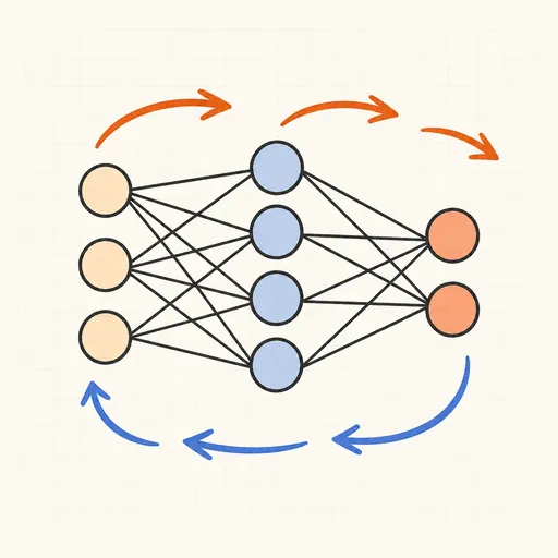
Backpropagation Step-by-Step
Walk through one forward and backward pass of a tiny neural network, number by number.

Handwritten Digit Recognizer
Draw a digit and watch a neural network trained on MNIST recognize it live in your browser.
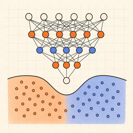
Neural Network Playground
Train a tiny neural network live in your browser and watch its decision boundary learn four classic datasets.

Activation Function Explorer
Compare sigmoid, tanh, ReLU and friends with their derivatives, and see why deep gradients vanish.
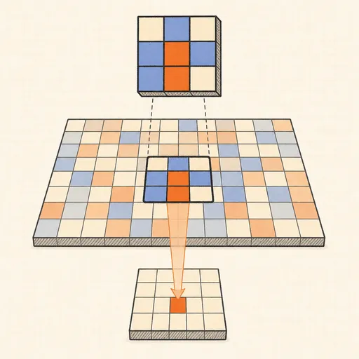
Convolution Filter Visualizer
Slide a 3×3 kernel over an image and watch convolution, ReLU and max-pooling build the output pixel by pixel.

Hopfield Network
Store pixel patterns in a Hopfield memory, corrupt them, and watch the network recall the original.