The SIR Epidemic Model, Explained
After reading this you will be able to write down the three SIR equations, predict whether an outbreak grows or dies out from a single number, and read the peak and final size off the curves the simulator draws.
What the model is, and one example
The SIR model tracks an epidemic by sorting everyone into three boxes. S is the number of people still susceptible, I is the number currently infected and able to infect others, and R is the number recovered (and now immune). People move only in one direction: S \to I \to R.
Here is the hook. Start with 999 susceptible people, 1 infected, an infection rate \beta = 0.3 per day and a recovery rate \gamma = 0.1 per day. That single infected person does not touch most of the town. Yet the number infected climbs to a peak near 106 people around day 41, then falls back to zero. When the dust settles about 941 people have been infected at some point and 59 never catch it. The disease runs out of fuel before it reaches everyone. That leftover pool of susceptibles is the counterintuitive result the model gives you for free.
When this model helps, and when it misleads
SIR is the right first tool when you want the shape of an epidemic: does it take off, how tall is the peak, when does it arrive, what fraction of people are hit. It captures the core feedback that as susceptibles run low, transmission slows even before anyone intervenes.
It is the wrong tool for anything that depends on structure. Real contact is not well-mixed: you meet your household far more than a stranger across town. Real diseases have an incubation delay (that needs an added Exposed box, giving SEIR). Real populations gain births and lose deaths, which can let a disease become endemic instead of burning out.
Do not read exact case counts off a toy SIR run as forecasts. A model with two constant rates and perfect mixing gives you qualitative behavior and rough scale, not a dated prediction. Treat 106 at the peak as "roughly a tenth of the town," not "exactly 106 people on day 41."
The equations and the intuition behind them
Let N = S + I + R be the fixed total. The model is three coupled differential equations:
New infections per day equal \beta times the fraction of contacts that land on a susceptible (S/N) times the number of infected people spreading it (I). The minus sign says susceptibles only leave.
The infected box gains exactly what S loses and drains at rate \gamma I as people recover. Here \beta is the effective transmission rate per infected person per day and \gamma is the recovery rate, so 1/\gamma is the average infectious period in days.
Recovered people accumulate the recoveries. Add the three right-hand sides and they cancel to zero, which is the algebra behind "constant population."
The one number that decides everything is the basic reproduction number:
It counts how many people one infected person infects in a fully susceptible population. Look back at dI/dt. Early on S \approx N, so the infected box grows when \beta - \gamma \gt 0, that is when R_0 \gt 1. Below 1 the outbreak shrinks from day one.
How the simulator solves it: RK4
These equations have no tidy closed-form solution, so the simulator steps forward in time numerically. It uses fourth-order Runge-Kutta (RK4), which is far more accurate than naive Euler stepping for the same step size. For a state y and step h, RK4 samples the slope four times and blends them:
Here k_1 is the slope at the start of the step, k_2 and k_3 are slopes evaluated at the midpoint using earlier estimates, and k_4 is the slope at the step's end. Averaging with weights 1, 2, 2, 1 cancels error terms up to order h^4. With a step of h = 0.1 day the error per step is tiny, so the animated curves match the true solution to well within a pixel.
A worked example reproducing the demo
One RK4 step for the default run
Use the demo defaults: N = 1000, S_0 = 999, I_0 = 1, R_0^{state} = 0, \beta = 0.3, \gamma = 0.1, step h = 1 day for a hand-sized number. First the reproduction number:
- Reproduction number: R_0 = 0.3 / 0.1 = 3. Above 1, so expect an outbreak.
- Slope at the start (k_1 for I): 0.3 \cdot 999 \cdot 1 / 1000 - 0.1 \cdot 1 = 0.2997 - 0.1 = 0.1997 infected per day. Positive, as predicted.
- Growth rate early on is \beta - \gamma = 0.2 per day, so I roughly doubles every \ln 2 / 0.2 \approx 3.47 days while susceptibles stay near 1000.
- Run the full RK4 loop to completion and the peak lands at about 106 infected near day 41.
The final epidemic size solves the transcendental relation S_\infty = S_0 \, e^{-R_0 (1 - S_\infty / N)}. Iterating for R_0 = 3 gives S_\infty \approx 59, so about 941 of the 1000 people are infected at some point and 59 escape.
Reading and interpreting the results
Three quantities carry most of the meaning.
- Peak infected
- The tallest point of the I curve. It sets the demand on hospitals. For the demo it is about 106 (10.6% of the town) at day 41.
- Peak timing
- How long you have before the wave crests. Larger R_0 pulls the peak earlier and higher. Halving \beta to 0.15 (so R_0 = 1.5) drops the peak to about 6% and pushes it past day 70. That delay-and-flatten is what "flattening the curve" means.
- Final size
- The share ever infected, read as (N - S_\infty)/N. At R_0 = 3 it is about 94%; at R_0 = 1.5 it drops to about 58%.
Vaccination shifts the starting point by moving people straight into R. Herd immunity is reached when the vaccinated fraction hits 1 - 1/R_0. For R_0 = 3 that is 1 - 1/3 \approx 0.667, so vaccinating two thirds of the town leaves so few susceptible contacts that a single case fails to grow.
Common mistakes
The first mistake is confusing \beta with R_0. A \beta of 0.3 sounds small, but paired with \gamma = 0.1 it means R_0 = 3, a strong epidemic. Always divide.
The second is expecting everyone to get infected. The final size is capped by the transcendental equation above, so at R_0 = 3 exactly 59 of 1000 people escape without any intervention. Herd immunity is not "no one susceptible left," it is "not enough susceptible contacts to sustain growth."
The third is misreading the peak as the end. At the peak dI/dt = 0, which happens precisely when S/N = \gamma/\beta = 1/R_0. For the demo that is S = 1000/3 \approx 333. Plenty of infection happens after the peak: the wave still has to drain.
Related simulators on this site
If you like watching coupled rates play out, the Predator-Prey Simulator uses the Lotka-Volterra equations, where two populations cycle instead of settling. For a different flavor of emergent behavior from simple local rules, the Traffic Jam Simulator shows jams forming on a ring road with no cause but density.
Frequently asked questions
What is R0 in plain terms?
It is the average number of people one infected person infects when everyone else is susceptible. It equals \beta / \gamma. Above 1 the outbreak grows, below 1 it fades. The demo value is 3.
Why does the epidemic stop before everyone is infected?
Because transmission slows as susceptibles run out. Once S/N drops below 1/R_0, each infected person infects fewer than one new person on average, so I falls. The remaining susceptibles never get their turn.
What fraction do I need to vaccinate?
To reach herd immunity, vaccinate 1 - 1/R_0 of the population. For R_0 = 3 that is about 66.7%; for R_0 = 5 it rises to 80%.
Why use RK4 instead of just adding the slope each step?
Plain Euler stepping accumulates error proportional to the step size and can overshoot the sharp peak. RK4 samples the slope four times per step and cancels error to order h^4, so with h = 0.1 day the curve is accurate to well under a pixel.
Can this model forecast a real outbreak?
Not reliably. It assumes perfect mixing, constant rates and no births or deaths. Use it to understand mechanisms and rough scale, not to predict exact case counts on a given date.
Related tools

Gerrymandering Sandbox
Draw the districts yourself and watch the same voters produce opposite election results.
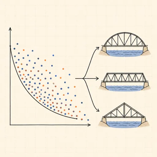
Pareto Frontier Evolution
Watch a genetic algorithm breed bridge designs and trace out the weight-vs-stiffness Pareto frontier, generation by generation.

Sailing & Tacking Simulator
Sail a boat against the wind — trim to the polar diagram, ride the shifts and race the optimal route.
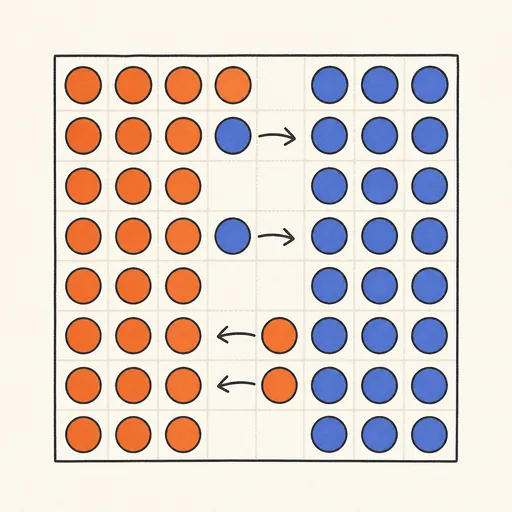
Schelling’s Segregation Model
Give agents a mild preference for similar neighbours and watch a mixed city sort itself into stark blocks.
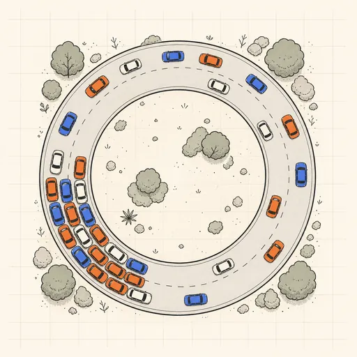
Traffic Jam Simulator
See phantom traffic jams appear from nothing on a ring road with the Nagel–Schreckenberg model.
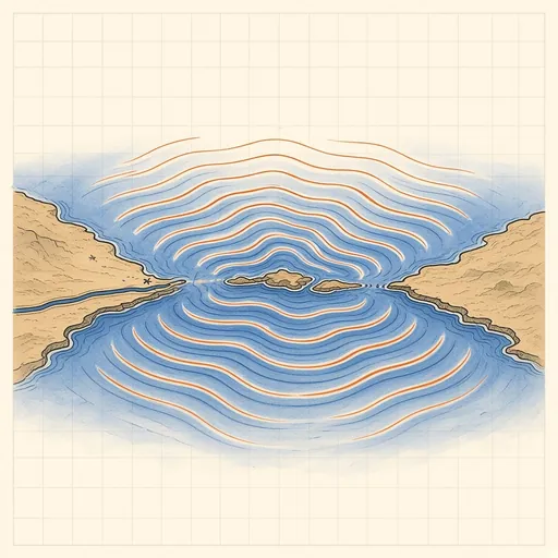
Tsunami Simulator
Set off an undersea earthquake anywhere and watch the tsunami cross real ocean floors — with arrival times at tide gauges around the world.