Particle Swarm Optimization, Explained
After reading this you will know how a swarm of candidate solutions searches a function using only its own memory and one shared best point, how to set the three coefficients so the swarm settles instead of exploding, and how to read the convergence curve to tell success from stagnation.
What particle swarm optimization does
Particle swarm optimization (PSO) minimizes a function by moving a population of candidate points around the search space. Each point is a particle. A particle carries a position x and a velocity v. On every step it nudges its velocity toward two attractors: the best position it has personally visited (its personal best), and the best position any particle in the swarm has visited (the global best). Then it moves.
That is the whole idea. No gradients, no derivatives, only function values. The swarm behaves like scouts spreading over terrain who periodically shout their best find to the group.
A quick example. Put 20 particles on the Rastrigin function, a bumpy grid of local minima with the true minimum at the origin where the value is 0. Scattered particles each fall into nearby dips. One particle lands closest to the center, say at value 3.2. That becomes the global best. Every other particle now feels a pull toward it, climbs out of its own shallow dip, and the swarm collapses toward the true minimum over a few dozen steps. The convergence curve, the best value found so far, drops from around 40 to below 0.01.
When to use it, and when not to
PSO earns its place when you cannot compute a gradient. The objective might be a black box, a simulation, a noisy measurement, or a function with flat and discontinuous regions. PSO only ever calls the function and compares numbers, so none of that troubles it.
It is also a reasonable first attempt on a low-dimensional problem, say 2 to 30 variables, where you want a decent answer without much tuning.
Do not reach for PSO when a gradient is cheap and the landscape is smooth. Gradient methods converge far faster there, often in tens of steps rather than hundreds. If your problem is smooth and continuous, compare against the methods in the Gradient Descent Visualizer before committing to a swarm. PSO also scales poorly in very high dimensions and gives no guarantee of finding the global minimum: it finds a good point, not a certified best point.
PSO is a heuristic. Run it twice with different random seeds and you will usually get two slightly different answers. That is expected. Report the best of several runs, not a single run.
The velocity update, symbol by symbol
Everything happens in one line, applied to every particle at every step:
Here v is the particle's current velocity and x its current position, both vectors. p_{best} is the best position this particle has visited so far, and g_{best} is the best position any particle has visited. The three coefficients control the mix:
- w (inertia)
- How much of the old velocity carries over. Large w keeps particles exploring; small w lets them settle.
- c_1 (cognitive)
- Pull toward the particle's own best find. This is the memory term.
- c_2 (social)
- Pull toward the shared global best. This is the only communication between particles.
- r_1, r_2
- Fresh uniform random numbers in
[0, 1], drawn independently for every particle and every dimension on every step. They add jitter so particles do not march in lockstep.
After computing v, optionally clamp each component to a velocity cap v_{max}, then move: x \leftarrow x + v. Finally re-evaluate the function, update p_{best} if the new point is better, and update g_{best} if it beats the swarm record.
The stability of the swarm depends almost entirely on w. If w \gt 1 the velocity term grows every step and speeds compound without limit. Below 1 the old velocity decays and the pulls toward the two bests keep the particle anchored. The standard stable choice is w \approx 0.72 with c_1 = c_2 \approx 1.49, a set derived by Clerc and Kennedy to keep the swarm on the edge of settling without stalling.
A worked example you can reproduce
Follow one particle through one step by hand, using the demo defaults: inertia w = 0.72, cognitive c_1 = 1.49, social c_2 = 1.49, on the sphere function f(x, y) = x^2 + y^2 whose minimum is 0 at the origin.
One particle, one step on the sphere
- Current state: position x = (3.0, -2.0), velocity v = (0.5, 0.5). Function value f = 3^2 + (-2)^2 = 13.
- Personal best so far: p_{best} = (2.0, -1.0), value 5.
- Global best across the swarm: g_{best} = (0.5, 0.5), value 0.5.
- Draw randoms. Suppose r_1 = 0.6 and r_2 = 0.8 (one pair per dimension is used here for clarity).
- Update the x-component of velocity:
v_x = 0.72 \cdot 0.5 + 1.49 \cdot 0.6 \cdot (2.0 - 3.0) + 1.49 \cdot 0.8 \cdot (0.5 - 3.0)That is 0.36 - 0.894 - 2.98 = -3.514.
- Update the y-component:
v_y = 0.72 \cdot 0.5 + 1.49 \cdot 0.6 \cdot (-1.0 + 2.0) + 1.49 \cdot 0.8 \cdot (0.5 + 2.0)That is 0.36 + 0.894 + 2.98 = 4.234.
- Move: x_{new} = (3.0 - 3.514, \; -2.0 + 4.234) = (-0.514, 2.234).
- New value: f = (-0.514)^2 + 2.234^2 = 0.264 + 4.991 = 5.256.
The particle jumped from 13 to about 5.26 in one step, overshooting the origin because the social pull was strong and no velocity cap trimmed the step. Since 5.26 is worse than its personal best of 5, p_{best} stays put. Over the next steps the shrinking inertia pulls the swing back toward the center.
Reading the convergence curve
The most useful readout is the best value found so far, plotted against the step number. A healthy run drops fast, then flattens as the swarm zeroes in. The curve below is a typical sphere run with 20 particles at the default coefficients.
Two shapes tell you something is off. A curve that plateaus early and high means the swarm converged on a local minimum and lost the diversity to escape. A curve that is jagged and refuses to settle means velocities are too large, usually because w is near or above 1 or the velocity cap is too generous.
Different functions produce different shapes. On Rosenbrock the swarm finds the curved valley within a handful of steps, so the value drops sharply, then crawls along the valley floor for a long time because the gradient along the valley is tiny. The curve shows a steep cliff followed by a long shallow slope.
How the coefficients change behavior
The table shows the qualitative effect of each dial. The numbers are illustrative outcomes on a 2D Rastrigin run with 20 particles over 60 steps.
| Change | Effect on swarm | Typical best value at step 60 |
|---|---|---|
| Default w=0.72, c_1=c_2=1.49 | Balanced explore then settle | 0.02 |
| Raise w to 1.05 | Velocities grow, swarm oscillates | 18.0 |
| Lower w to 0.3 | Settles fast, may trap early | 4.5 |
| Raise c_2 to 3.0 | Rushes to global best, loses diversity | 3.1 |
| Raise c_1 to 3.0 | Particles chase own memory, slow to agree | 2.4 |
The pattern: w controls stability, the balance of c_1 and c_2 controls the tug of war between individual exploration and group agreement. Rastrigin punishes a swarm that agrees too fast, because agreeing early means agreeing on a shallow dip that is not the true minimum.
Common mistakes
The failures below account for most disappointing runs.
Setting inertia at or above 1 is the classic error. The velocity term then feeds on itself: with w = 1.05 a velocity of 2 becomes at least 2.1 before any pull is added, and the excess compounds every step until particles fly off the map.
No velocity cap on a wide search space. Without a cap, the first few steps on a large domain can throw particles thousands of units away, and they waste time flying back. A cap of roughly 10 to 20 percent of the domain width keeps steps sane.
Too few particles in a bumpy landscape. On Rastrigin or Himmelblau, a swarm of 5 particles often lands entirely inside one basin and never sees the others. Twenty to forty particles give enough coverage to compare basins.
Reading a single run as the truth. PSO is stochastic. One run that stalls at 3.1 does not mean the method failed; three more runs may all reach 0.02. Judge by the best of several.
Confusing "found the valley" with "solved it." On Rosenbrock the value can sit at 0.5 for fifty steps while the swarm inches along the valley. That is progress, not failure. Give it more steps.
Related tools on this site
PSO is one of several search strategies worth comparing side by side. If your objective is smooth and you can compute a gradient, the Gradient Descent Visualizer races SGD, Momentum, RMSProp and Adam across the same kind of contour maps and will usually beat PSO on those landscapes. For a combinatorial problem where positions are discrete tours rather than continuous points, the Simulated Annealing TSP tool shows a different escape-from-local-minima strategy driven by a cooling schedule. If instead of optimizing you want to track a moving state through noise, the Kalman Filter Visualizer covers the linear filtering case.
Frequently asked questions
How many particles should I use?
For 2D problems, 20 to 40 is a common range. Fewer than 10 risks missing basins on bumpy functions like Rastrigin. More than 50 rarely helps in low dimensions and just costs more function evaluations per step. Scale up with dimensionality if you go higher.
Does PSO find the global minimum?
No guarantee. PSO is a heuristic that often finds the global minimum on friendly problems but can converge to a local one. On the sphere function it reliably reaches the true minimum near 0; on Himmelblau it may settle into any of the four equal minima. Run it several times and keep the best.
Why does the swarm explode when I raise the inertia?
Inertia multiplies the old velocity each step. When w \lt 1 that old velocity decays; when w \ge 1 it grows or holds, and the added pulls keep pushing it larger. The result is velocities that increase without bound, so positions oscillate with growing amplitude and never settle. Keep w around 0.72.
Can PSO handle noisy or discontinuous functions?
Yes. PSO uses only function values, never derivatives, so a jump discontinuity or a noisy evaluation does not break the update rule. Gradient methods, by contrast, need a well-defined slope. This is the main practical reason to choose PSO over gradient descent.
What does clicking the map do?
It reseeds the swarm around the clicked point. This lets you test how sensitive the outcome is to the starting region: seed near a shallow local dip on Rastrigin and watch whether the swarm still escapes to the center, or seed inside Rosenbrock's valley and watch how slowly it crawls.
Related tools
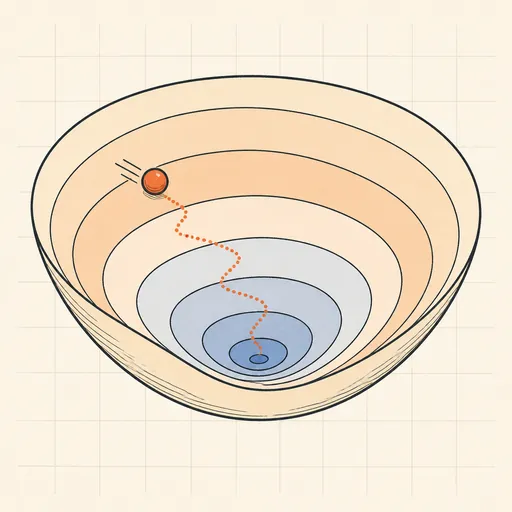
Gradient Descent Visualizer
Race SGD, Momentum, RMSProp and Adam across contour maps of five classic loss landscapes.

Kalman Filter Visualizer
Track a moving target through noisy measurements with a full linear Kalman filter.
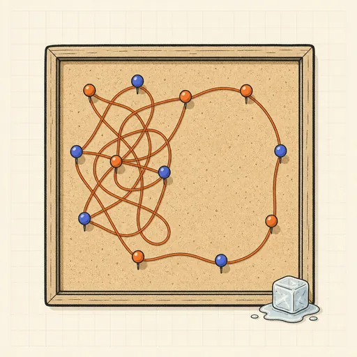
Simulated Annealing TSP
Watch simulated annealing untangle a travelling-salesman tour as the temperature falls.
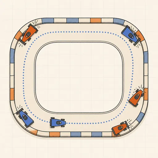
AI Learns to Drive (Neuroevolution)
Watch a population of neural-network cars evolve from crashing into corners to lapping a race track.
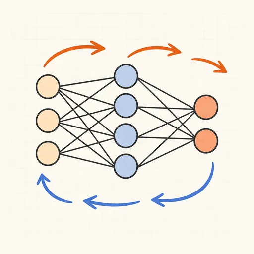
Backpropagation Step-by-Step
Walk through one forward and backward pass of a tiny neural network, number by number.
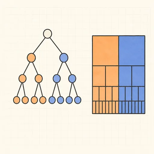
Decision Tree Builder
Grow a CART decision tree split by split and watch the partition map and tree diagram build together.