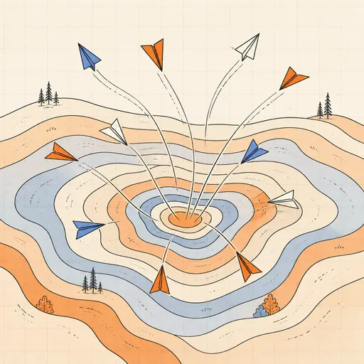
Particle Swarm Optimization
Particle swarm optimization searches a function with a flock of candidate solutions: each particle keeps a velocity that blends its own momentum (inertia w), a pull toward the best point it has personally found (cognitive c1) and a pull toward the best point any particle has found (social c2). Choose among sphere, Rastrigin, Rosenbrock, Ackley and Himmelblau, drawn as a shaded contour map, and watch blue particles with velocity trails sweep over it — faint green dots mark personal bests and an orange star the global best. Tune the swarm size, the three coefficients and the velocity cap, follow the convergence curve of the best value found, and click anywhere on the map to reseed the swarm around that spot.
Runs 100% in your browser — models are trained and computed locally on your device.
Read the full guide to this tool
Notes
- Velocity update per particle: v ← w·v + c1·r1·(pbest − x) + c2·r2·(gbest − x) with fresh uniform randoms r1, r2 each step — the only communication is the shared global best.
- The standard stable choice is w ≈ 0.72 with c1 = c2 ≈ 1.49; push the inertia above 1 and velocities grow without bound, so the swarm oscillates and diverges instead of settling.
- Rastrigin’s grid of local minima shows why the social term matters, while Rosenbrock’s curved valley is easy to enter but slow to traverse — the swarm finds the valley fast and then crawls.
- PSO uses no gradients at all, only function values, so it works unchanged on discontinuous or noisy objectives.
- Runs 100% in your browser — models are trained and computed locally on your device.
Related tools
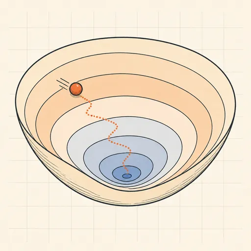
Gradient Descent Visualizer
Race SGD, Momentum, RMSProp and Adam across contour maps of five classic loss landscapes.
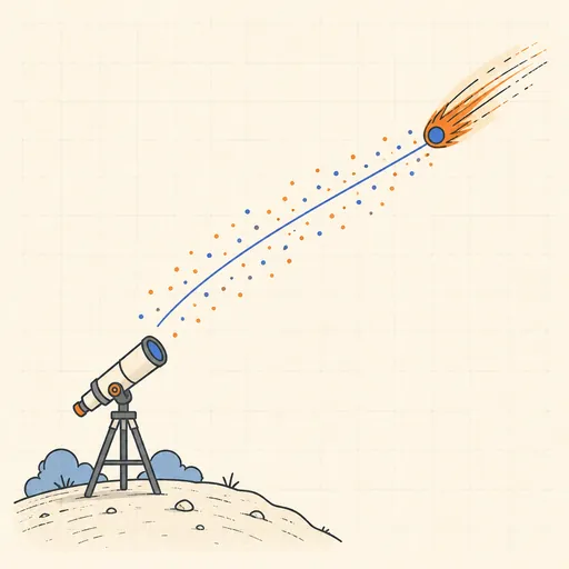
Kalman Filter Visualizer
Track a moving target through noisy measurements with a full linear Kalman filter.
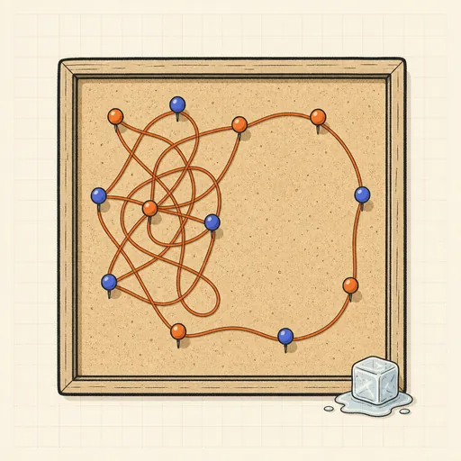
Simulated Annealing TSP
Watch simulated annealing untangle a travelling-salesman tour as the temperature falls.
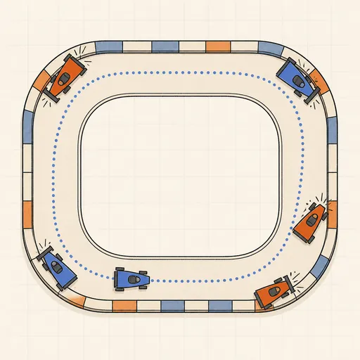
AI Learns to Drive (Neuroevolution)
Watch a population of neural-network cars evolve from crashing into corners to lapping a race track.
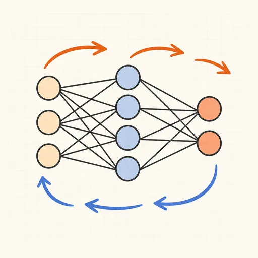
Backpropagation Step-by-Step
Walk through one forward and backward pass of a tiny neural network, number by number.
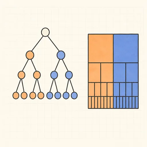
Decision Tree Builder
Grow a CART decision tree split by split and watch the partition map and tree diagram build together.