The Kalman Filter, Explained
After reading this you will know how a Kalman filter blends a motion model with noisy sensor readings, be able to run the five update equations by hand on a small example, and read the uncertainty ellipse and RMS numbers the visualizer draws.
What the Kalman filter does
A Kalman filter estimates a hidden state you cannot measure directly, using measurements that are noisy and possibly incomplete. In the visualizer the hidden state is a target's position and velocity, written as the vector x = (p_x, p_y, v_x, v_y). The sensor reports only a noisy position, not velocity. The filter still recovers a smooth velocity estimate because it carries a model of how position and velocity relate over time.
Here is the hook. Suppose the true target sits at x = 100 and moves right at 2 pixels per step. The sensor reports positions like 103, 97, 101, 96, 104: scattered by about 3 pixels each. If you just plotted the raw readings, your track would jitter by that same 3 pixels. A Kalman filter that knows the target moves smoothly will produce a track that stays within roughly 1 pixel of truth, because it treats each new reading as a correction to a prediction rather than as the whole answer.
The blue line in the tool is the truth, the orange line is the filtered estimate, and the gray dots are the raw measurements. The status line reports two root-mean-square errors so you can confirm the filtered track beats the raw dots.
When to use it, and when not
Reach for a Kalman filter when three things hold. First, you have a state that evolves in a way you can write as a linear equation, such as constant velocity or constant acceleration. Second, your measurements are a linear function of that state plus roughly Gaussian noise. Third, you want a running estimate that updates cheaply as each measurement arrives, without storing the whole history.
The constant-velocity model in the tool assumes velocity changes only through random nudges. That fits a target drifting across a screen. It fits a car on a highway between lane changes. It does not fit a target that swerves hard, unless you raise the process noise to admit that the model is wrong.
The filter is provably optimal only when the true system really is linear with Gaussian noise. If the target turns sharply and you have set the process noise low, the estimate will lag behind by several steps. That is not a bug. You told the filter to trust its straight-line model, so it did.
For nonlinear systems (a robot with steering angle, a satellite in orbit) you need the extended or unscented variants. Those linearize around the current estimate. The plain filter here is the foundation for all of them.
The five equations and what each one means
Every step runs a predict phase and an update phase. The predict phase pushes the estimate forward in time using the model. The update phase pulls it back toward the new measurement.
Here x is the state estimate and P is its covariance, a matrix describing how uncertain each component is and how the errors correlate. The matrix F is the state transition: for constant velocity it adds velocity times the time step to position. The matrix Q is the process noise, the amount of new uncertainty the model injects each step. Bigger Q means you distrust your own model.
The matrix H maps state to measurement space: here it picks out p_x and p_y and ignores velocity. The matrix R is the measurement noise. The Kalman gain K is the blend ratio. When R is large (a bad sensor), K shrinks toward zero and you barely move. When P^- is large (you are unsure), K grows toward one and you snap to the measurement.
The term z - H x^- is the innovation: the gap between the measurement z and what you predicted. The green line in the tool draws exactly this gap. The covariance P always shrinks in the update, which is why the ellipse contracts right after each accepted measurement.
A worked example you can reproduce
Run the demo with the field defaults. To keep the arithmetic checkable by hand, follow one axis only, treating position and velocity along x as a 2-vector (p, v) with time step \Delta t = 1.
One dimension, three steps
Start with x = (100, 2) and covariance P = \begin{bmatrix} 10 & 0 \\ 0 & 4 \end{bmatrix}. Use F = \begin{bmatrix} 1 & 1 \\ 0 & 1 \end{bmatrix}, measurement matrix H = [1, 0], measurement noise R = 9 (a standard deviation of 3 pixels), and a small process noise Q = \begin{bmatrix} 0.1 & 0 \\ 0 & 0.1 \end{bmatrix}.
- Predict. x^- = F x = (100 + 2, 2) = (102, 2). The predicted position variance is P^-_{11} = P_{11} + 2 P_{12} + P_{22} + Q_{11} = 10 + 0 + 4 + 0.1 = 14.1.
- Gain. The innovation variance is S = P^-_{11} + R = 14.1 + 9 = 23.1. The position gain is K_1 = P^-_{11} / S = 14.1 / 23.1 = 0.6104.
- Update. A measurement arrives at z = 103. The innovation is 103 - 102 = 1. The corrected position is 102 + 0.6104 \times 1 = 102.61. The position variance drops to (1 - 0.6104) \times 14.1 = 5.494.
Notice two things. The estimate moved only 0.61 pixels toward a measurement that was 1 pixel off, because the sensor is noisy. And the variance fell from 14.1 to 5.49, so the very next prediction will be more confident. Repeat the predict and update with z = 97, then z = 101, and the gain settles toward a steady value near 0.5 while the estimate tracks the true motion far more smoothly than the raw readings.
Reading the ellipse and the RMS numbers
The orange ellipse is the 2σ contour of the position part of P. Roughly 95 percent of the time the true position lies inside it, if your noise settings match reality. Its size is the filter's honest statement of how much it knows. Its tilt shows correlation between the x and y errors.
Watch the ellipse during a measurement dropout. With no measurement, only the predict step runs, so P grows by Q every step and never shrinks. Over ten missed frames the position variance can climb from 5 to well over 50, and the ellipse swells to match. The moment a measurement returns, the update step slams it back down.
The chart below shows position variance across a run with a dropout between steps 20 and 30.
The status line's RMS comparison is the honest scoreboard. With R = 9 the raw measurements carry an RMS position error near 3.0 pixels, because their standard deviation is 3. A well-tuned filter here typically reports a filtered RMS near 1.3 pixels. If your filtered RMS is worse than the raw RMS, your model is wrong: the target is turning harder than your Q allows.
Common mistakes
The most frequent error is mistuning Q and R. These are variances, not standard deviations. A sensor with a 3-pixel spread needs R = 9, not R = 3. Set R = 3 and the filter trusts the sensor more than it should, so the track jitters.
A second error is starting with a tiny initial P. If you claim near-perfect confidence at step 0 but your initial guess is off, the gain stays low and the filter takes many steps to recover. Start P large when the initial state is a guess.
Tune in this order. First set R from the known sensor spread. Then raise Q until the filter keeps up with real maneuvers without inheriting obvious noise. If the innovation (green line) is consistently large and one-sided, your model is biased, not just noisy.
A third error is expecting the ellipse to mean the estimate is wrong by that much. The ellipse is the filter's belief given its noise settings. If those settings are optimistic, the true error can be larger than the ellipse suggests. Check the belief against the actual RMS.
Related tools
The Kalman filter estimates a state under a fixed model. If you instead want to fit model parameters by minimizing a loss surface, the Gradient Descent Visualizer shows how optimizers descend classic loss landscapes. For combinatorial search rather than continuous estimation, the Simulated Annealing TSP and the Particle Swarm Optimization tools show two population-free and population-based ways to hunt for a global minimum.
Frequently asked questions
Why does the filter track velocity when the sensor only reports position?
The transition matrix F couples position and velocity: next position equals current position plus velocity. Because the filter carries the correlation between them in P, a run of position measurements that keep rising by 2 forces the velocity estimate toward 2. You never measure velocity, you infer it from consistent position change.
What is the difference between Q and R in one sentence?
Q says how wrong your motion model is, and R says how wrong your sensor is; the gain is the ratio that decides which one to trust at each step.
Why does the ellipse grow without bound during a dropout?
Only the predict step runs, and it adds Q to P every step with nothing to counter it. In the chart above the variance climbs about 4.6 per step, from 5.2 to 51.7 over ten missed frames, and keeps climbing as long as measurements stay away.
Is the filter guaranteed to beat the raw measurements?
For a truly linear system with Gaussian noise and correct Q and R, yes: the Kalman filter is the minimum-variance estimator, so its RMS is at most the raw RMS. If your filtered RMS is worse, an assumption is broken, usually a maneuver your Q is too small to admit.
What happens if I set Q to exactly zero?
The filter believes its model perfectly. The gain shrinks toward zero over time, the estimate stops responding to measurements, and any real maneuver leaves the track stuck on the old straight line. A small positive Q keeps the filter alive.
Related tools
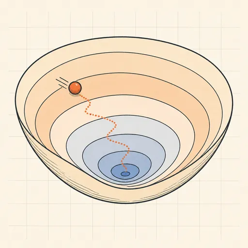
Gradient Descent Visualizer
Race SGD, Momentum, RMSProp and Adam across contour maps of five classic loss landscapes.
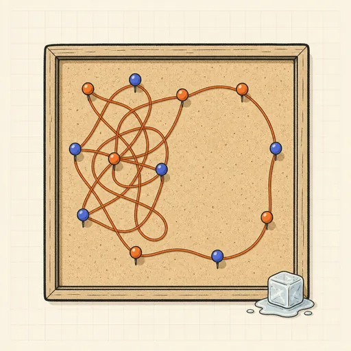
Simulated Annealing TSP
Watch simulated annealing untangle a travelling-salesman tour as the temperature falls.
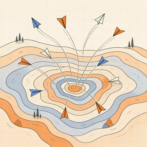
Particle Swarm Optimization
Fly a swarm of particles across classic test functions and watch it converge on the minimum.
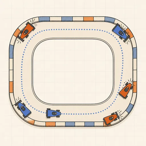
AI Learns to Drive (Neuroevolution)
Watch a population of neural-network cars evolve from crashing into corners to lapping a race track.
Backpropagation Step-by-Step
Walk through one forward and backward pass of a tiny neural network, number by number.
Decision Tree Builder
Grow a CART decision tree split by split and watch the partition map and tree diagram build together.